install.packages("jpstat")Note: This article is translated from my Japanese article.
About this article
This article is Day 12 of the “R Advent Calendar 2022”.
Last year marked 150 years since the establishment of government statistics in Japan (Chronology of statistics in the Heisei and Reiwa eras). More recently, it has become possible to browse and download a wide variety of government statistical data through the Portal Site of Official Statistics of Japan (e-Stat).
e-Stat also provides a convenient API (see the usage guide here; please check the terms of use beforehand. Before using the API, you also need to complete user registration).
In this article, I introduce how to use the e-Stat API efficiently with R’s jpstat package.
About e-Stat
e-Stat organizes a wide variety of government statistical databases. Here, let’s take a look at the database on sleep duration from the results of the 2015 National Health and Nutrition Survey.
Opening the database displays a statistical table as shown below, and you can download the data from the “Download” button in the upper right.
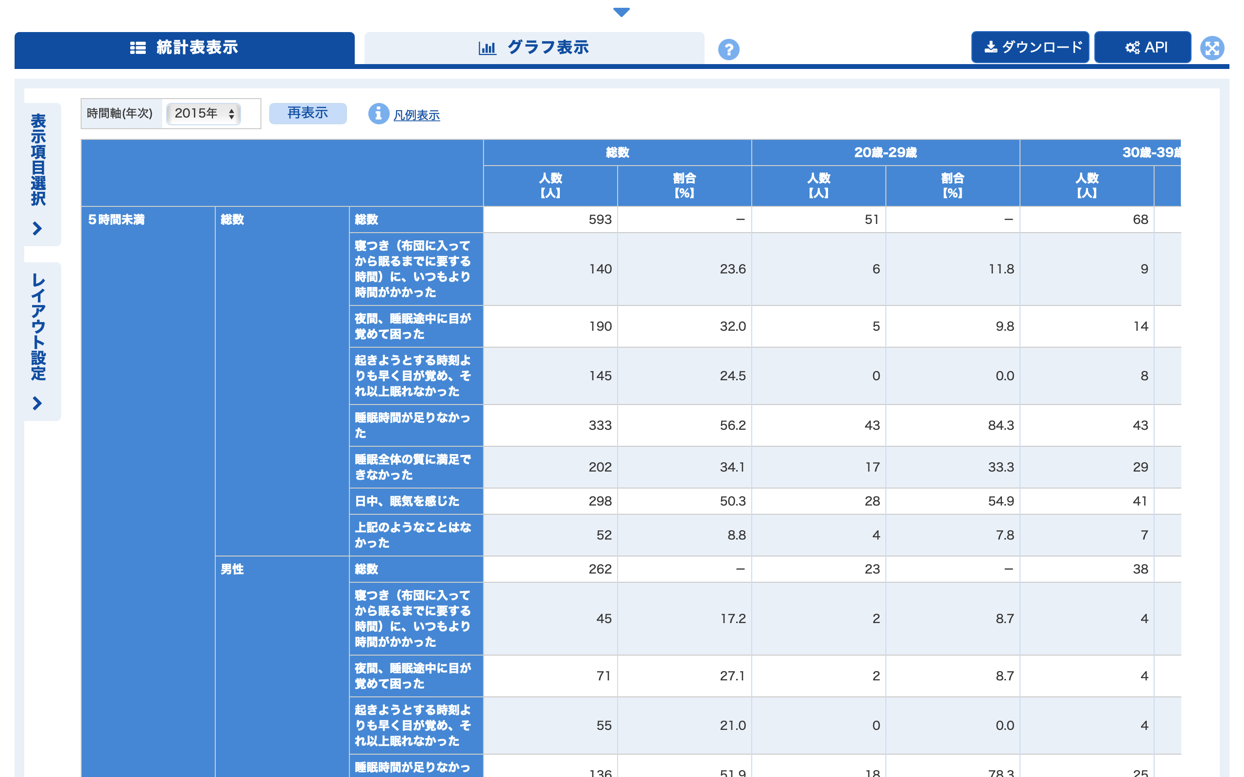
Clicking the “Select display items” button in the upper left lets you choose which data items (age group, sex, etc.) to display.
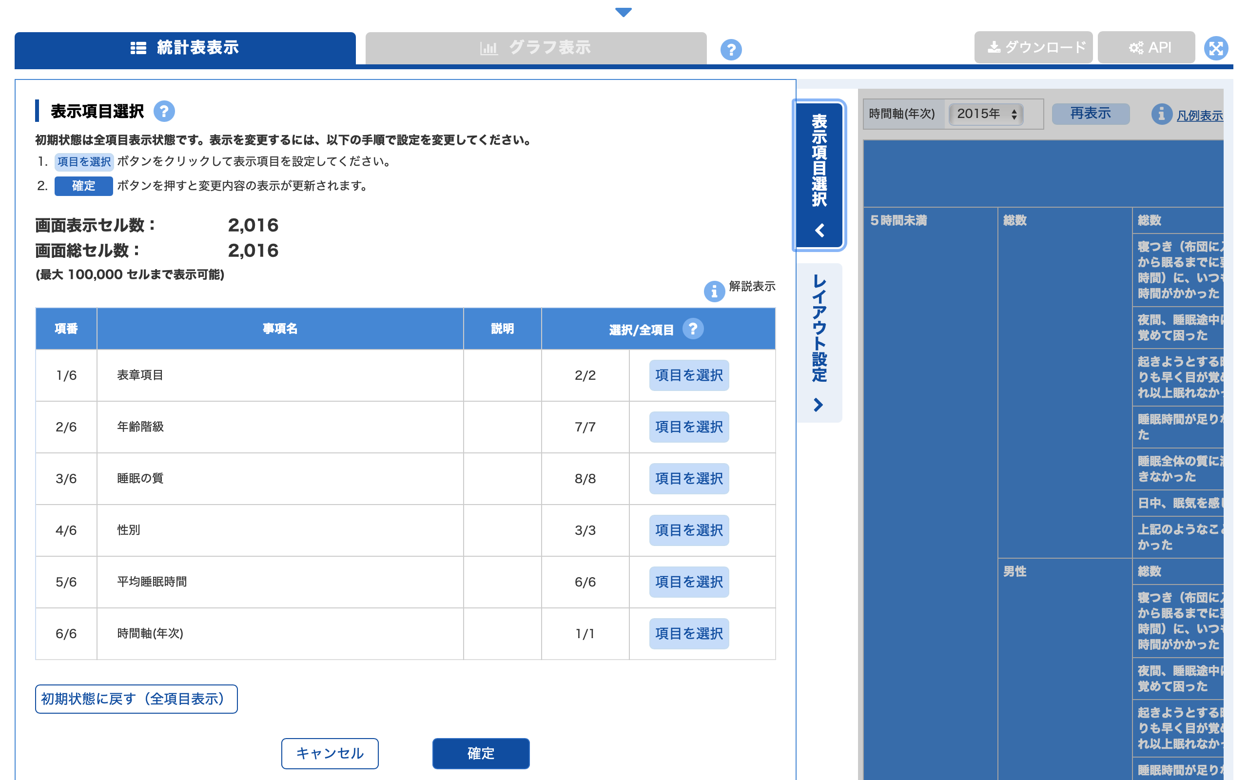
For example, if you want to select age groups, clicking the “Select items” button for age group brings up a screen like the one below, where you can choose the age groups.
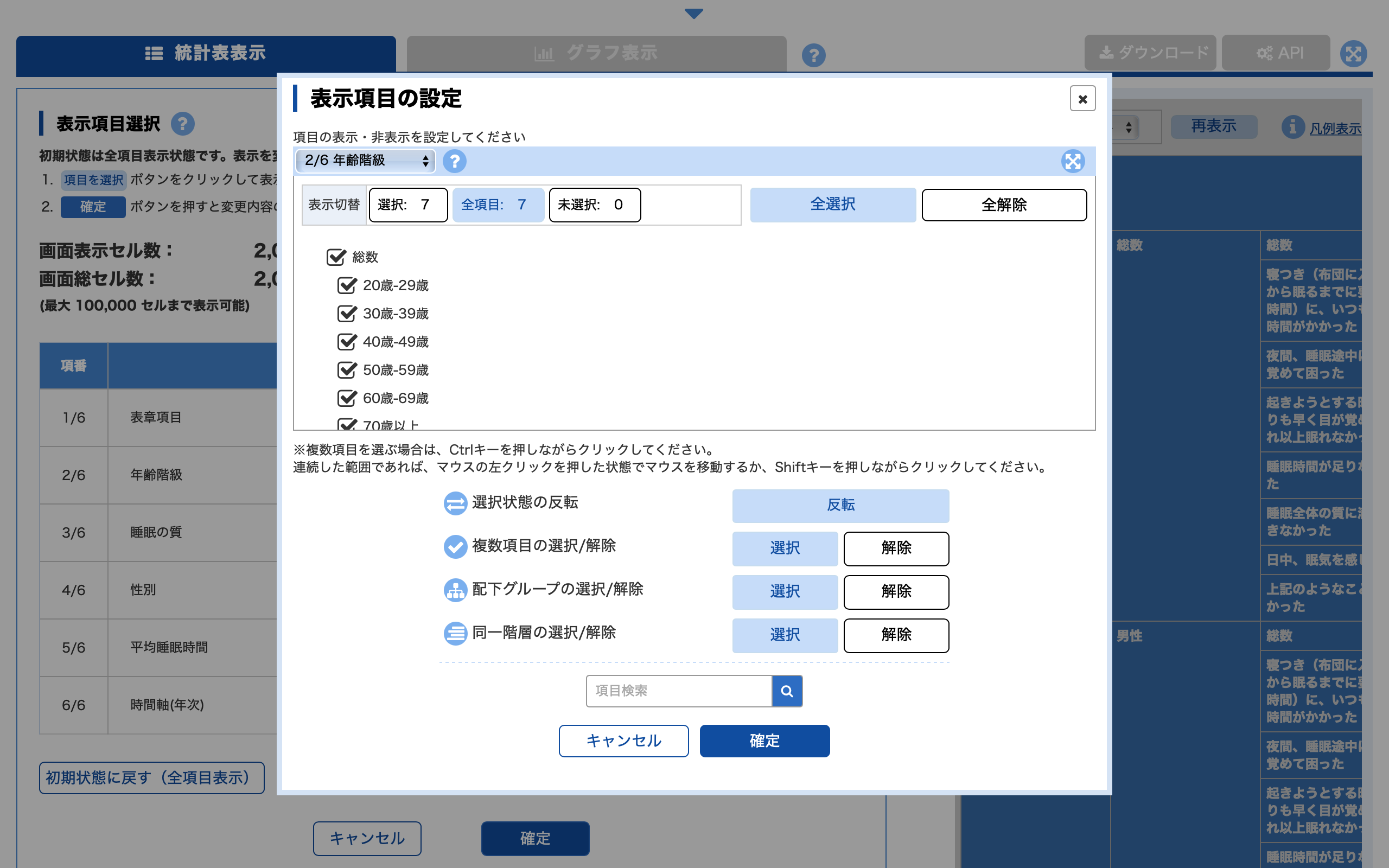
After selecting the display items, clicking the “Download” button lets you download only the data for the selected items.
In this way, e-Stat makes it easy to extract and download data. However, if you want to improve the reproducibility of your data-retrieval work or make programmatic data extraction and retrieval more efficient, using the e-Stat API is recommended.
Using the e-Stat API with the jpstat package
To perform, via the e-Stat API, the same data extraction and download process described above for e-Stat, you need to follow steps like these.
- Retrieve metadata and set parameters: retrieve and select the display item data, and set the API parameters corresponding to the selected items
- Retrieve statistical data: retrieve the selected data and format it into a table
The jpstat package was developed to carry out this series of tasks efficiently in R1. The jpstat package can be installed from CRAN.
Here, with the goal of plotting sleep duration by sex and age group, let’s retrieve data from the sleep duration database (2015) introduced above. First, load the required packages.
library(tidyverse)
library(jpstat)
Step 1: Display and extract the metadata (display items)
To use the e-Stat API, you first need to complete user registration and obtain an application ID called appId2.
By passing the appId and the database URL (or the statistical table ID, statsDataId) to the estat() function, you can retrieve the metadata (display items)3.
First, let’s look at the metadata for “age group (cat01)” ( cat01 is the classification name used in the API). The activate() function displays the metadata, and the filter() function lets you select items. Here, since we only need the data broken down by age group, we remove the “total” data4.
By using the pipe operator |>, you can continue extracting metadata for parameters other than cat01 as shown below. Here, we extract the number of respondents by sex, age group, and sleep duration.
# Replace this with your own appId
Sys.setenv(ESTAT_API_KEY = "Your appId")
estat_sleeptime_2015 <- estat(statsDataId = "https://www.e-stat.go.jp/dbview?sid=0003224282")# View and select the metadata
estat_sleeptime_2015 |>
activate(cat01) |>
filter(name != "総数")# ☐ tab: 表章項目 [2] <code, name, level, unit>
# ☒ cat01: 年齢階級 [6] <code, name, level, parentCode>
# ☐ cat02: 睡眠の質 [8] <code, name, level, parentCode>
# ☐ cat03: 性別 [3] <code, name, level, parentCode>
# ☐ cat04: 平均睡眠時間 [6] <code, name, level, parentCode>
# ☐ time: 時間軸(年次) [1] <code, name, level>
#
# A tibble: 6 × 5
# Stickers: .estat_rowid
.estat_rowid code name level parentCode
* <int> <chr> <chr> <chr> <chr>
1 2 160 20歳-29歳 2 100
2 3 170 30歳-39歳 2 100
3 4 180 40歳-49歳 2 100
4 5 190 50歳-59歳 2 100
5 6 210 60歳-69歳 2 100
6 7 220 70歳以上 2 100 estat_sleeptime_2015_filtered <- estat_sleeptime_2015 |>
# Tabulation item
activate(tab) |>
filter(name == "人数") |>
# Age group
activate(cat01) |>
filter(name != "総数") |>
# Sleep quality
activate(cat02) |>
filter(name == "総数") |>
# Sex
activate(cat03) |>
filter(name %in% c("男性", "女性"))Step 2: Retrieve (download) the statistical data
Applying collect() after extracting the data retrieves the statistical data. You can also use the n argument of collect() to name the column of retrieved data. Here, we name it "person".
Looking at the retrieved data data_sleeptime_2015, you can see it has many columns, making it hard to work with for analysis. In Step 2+α, I explain how to retrieve and reshape the data at the same time.
data_sleeptime_2015 <- estat_sleeptime_2015_filtered |>

  # Retrieve the data and convert to numeric
  collect(n = "person") |>
  mutate(person = parse_number(person))
The total number of data is 72.knitr::kable(head(data_sleeptime_2015, 10))| tab_code | tab_name | tab_level | tab_unit | cat01_code | cat01_name | cat01_level | cat01_parentCode | cat02_code | cat02_name | cat02_level | cat02_parentCode | cat03_code | cat03_name | cat03_level | cat03_parentCode | cat04_code | cat04_name | cat04_level | cat04_parentCode | time_code | time_name | time_level | person |
|---|---|---|---|---|---|---|---|---|---|---|---|---|---|---|---|---|---|---|---|---|---|---|---|
| 100 | 人数 | 人 | 160 | 20歳-29歳 | 2 | 100 | 100 | 総数 | 1 | NA | 110 | 男性 | 2 | 100 | 110 | 5時間未満 | 2 | 100 | 2015000000 | 2015年 | 1 | 23 | |
| 100 | 人数 | 人 | 160 | 20歳-29歳 | 2 | 100 | 100 | 総数 | 1 | NA | 110 | 男性 | 2 | 100 | 120 | 5時間以上6時間未満 | 2 | 100 | 2015000000 | 2015年 | 1 | 86 | |
| 100 | 人数 | 人 | 160 | 20歳-29歳 | 2 | 100 | 100 | 総数 | 1 | NA | 110 | 男性 | 2 | 100 | 130 | 6時間以上7時間未満 | 2 | 100 | 2015000000 | 2015年 | 1 | 88 | |
| 100 | 人数 | 人 | 160 | 20歳-29歳 | 2 | 100 | 100 | 総数 | 1 | NA | 110 | 男性 | 2 | 100 | 140 | 7時間以上8時間未満 | 2 | 100 | 2015000000 | 2015年 | 1 | 37 | |
| 100 | 人数 | 人 | 160 | 20歳-29歳 | 2 | 100 | 100 | 総数 | 1 | NA | 110 | 男性 | 2 | 100 | 150 | 8時間以上9時間未満 | 2 | 100 | 2015000000 | 2015年 | 1 | 19 | |
| 100 | 人数 | 人 | 160 | 20歳-29歳 | 2 | 100 | 100 | 総数 | 1 | NA | 110 | 男性 | 2 | 100 | 160 | 9時間以上 | 2 | 100 | 2015000000 | 2015年 | 1 | 3 | |
| 100 | 人数 | 人 | 160 | 20歳-29歳 | 2 | 100 | 100 | 総数 | 1 | NA | 120 | 女性 | 2 | 100 | 110 | 5時間未満 | 2 | 100 | 2015000000 | 2015年 | 1 | 28 | |
| 100 | 人数 | 人 | 160 | 20歳-29歳 | 2 | 100 | 100 | 総数 | 1 | NA | 120 | 女性 | 2 | 100 | 120 | 5時間以上6時間未満 | 2 | 100 | 2015000000 | 2015年 | 1 | 106 | |
| 100 | 人数 | 人 | 160 | 20歳-29歳 | 2 | 100 | 100 | 総数 | 1 | NA | 120 | 女性 | 2 | 100 | 130 | 6時間以上7時間未満 | 2 | 100 | 2015000000 | 2015年 | 1 | 94 | |
| 100 | 人数 | 人 | 160 | 20歳-29歳 | 2 | 100 | 100 | 総数 | 1 | NA | 120 | 女性 | 2 | 100 | 140 | 7時間以上8時間未満 | 2 | 100 | 2015000000 | 2015年 | 1 | 55 |
Step 2+α: Retrieve and reshape the data at the same time
When you retrieve e-Stat data with jpstat, columns (such as cat01_code and cat01_name) are created from the parameter names (such as cat01) combined with the column name for each item (code, name, etc.).
In jpstat, you can tidy up the data by renaming parameters with the rekey() function and selecting columns per item with the select() function5. Writing the code as below produces a nicely tidied dataset.
data_sleeptime_2015 <- estat_sleeptime_2015 |>
  activate(tab) |>
  filter(name == "人数") |>
  select() |>

  activate(cat01) |>
  rekey("ageclass") |>
  filter(name != "総数") |>
  select(name) |>

  activate(cat02) |>
  filter(name == "総数") |>
  select() |>

  activate(cat03) |>
  rekey("sex") |>
  filter(name %in% c("男性", "女性")) |>
  select(name) |>

  activate(cat04) |>
  rekey("sleeptime") |>
  select(name) |>

  activate(time) |>
  select() |>

  collect(n = "person") |>
  mutate(person = parse_number(person))
The total number of data is 72.knitr::kable(head(data_sleeptime_2015, 10))| ageclass_name | sex_name | sleeptime_name | person |
|---|---|---|---|
| 20歳-29歳 | 男性 | 5時間未満 | 23 |
| 20歳-29歳 | 男性 | 5時間以上6時間未満 | 86 |
| 20歳-29歳 | 男性 | 6時間以上7時間未満 | 88 |
| 20歳-29歳 | 男性 | 7時間以上8時間未満 | 37 |
| 20歳-29歳 | 男性 | 8時間以上9時間未満 | 19 |
| 20歳-29歳 | 男性 | 9時間以上 | 3 |
| 20歳-29歳 | 女性 | 5時間未満 | 28 |
| 20歳-29歳 | 女性 | 5時間以上6時間未満 | 106 |
| 20歳-29歳 | 女性 | 6時間以上7時間未満 | 94 |
| 20歳-29歳 | 女性 | 7時間以上8時間未満 | 55 |
Bonus: Plotting the retrieved data
Finally, let’s plot the 2015 sleep duration data by sex and age group that we retrieved. The plot shows that the pattern of sleep duration by age group differs between men and women.
data_sleeptime_2015 |>
  mutate(ageclass_name = as_factor(ageclass_name),
         sex_name = as_factor(sex_name),
         sleeptime_name = as_factor(sleeptime_name)) |>
  group_by(ageclass_name, sex_name) |>
  mutate(prop = person / sum(person)) |>
  ungroup() |>
  ggplot(aes(ageclass_name, prop,
             fill = fct_rev(sleeptime_name))) +
  geom_col() +
  geom_text(aes(label = if_else(prop > 0.05,
                                scales::label_percent(accuracy = 1)(prop),
                                "")),
            position = position_stack(vjust = 0.5)) +
  scale_x_discrete("Age group") +
  scale_y_continuous("Proportion",
                     labels = scales::label_percent(accuracy = 1)) +
  scale_fill_brewer("Sleep duration",
                    palette = "Spectral") +
  facet_wrap(~ sex_name) +
  guides(x = guide_axis(n.dodge = 2))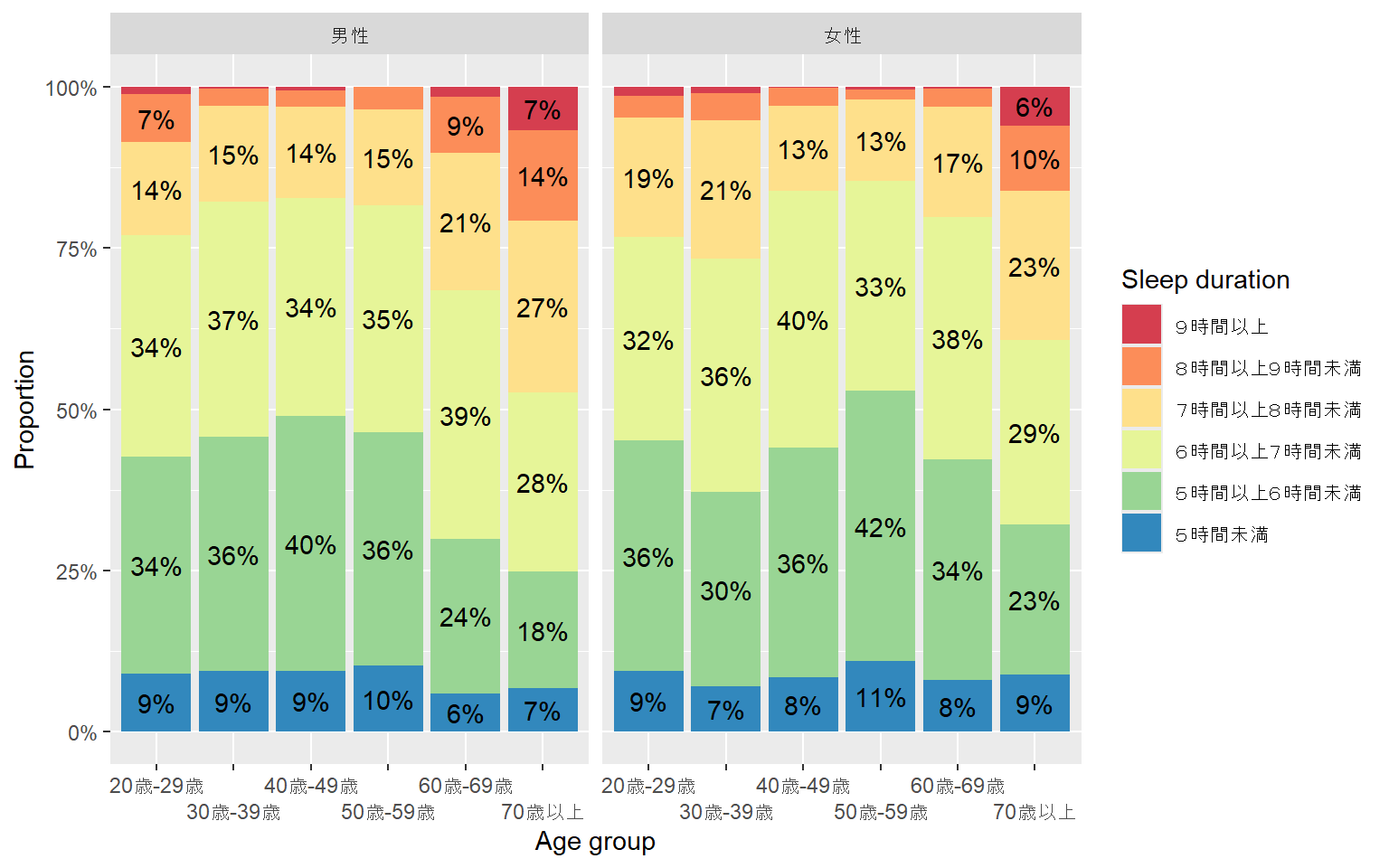
Summary
In this article, I introduced how to efficiently retrieve Japanese statistical data using the e-Stat API and the jpstat package.
Retrieving statistical data in R improves the reproducibility and efficiency of your work. The jpstat package is also convenient because it lets you retrieve and reshape data at the same time. I encourage you to give it a try.
Footnotes
The e-Stat API provides a variety of other functionality besides metadata retrieval and statistical data retrieval (see the API specification).↩︎
To obtain an application ID, you need to register a URL. If you are not going to use it on a public site, it is recommended that you enter a local address such as
http://test.localhost/(for details, see the usage guide).↩︎Clicking the “API” button in the upper right of an e-Stat page displays the corresponding API query. You can also retrieve metadata by directly entering the
statsDataIdfound in that query.↩︎Note, however, that each parameter has an upper limit of 100 items, so if filtering would still leave a large number of items, it is recommended to select all items without filtering.↩︎
You can also use the
select()function to drop all columns for a given item. This is convenient when you want to remove items that aren’t needed for analysis, such as when only the “total” is selected.↩︎