Loading packages, etc.
library(tidyverse)
library(fs)
library(arrow)
library(readxl)
library(jpstat)

theme_set(theme_light())

dir_create("quantify-vote-disparity-between-generations")Note: This article is translated from my Japanese article.
Since it’s currently election season1, I’d like to use open data to quantify the “vote-value disparity,” an issue that often comes up.
The “vote-value disparity” usually refers to the fact that the number of eligible voters per elected representative differs by region (electoral district) — in other words, the number of votes needed to elect one representative differs by region. For example, in the 2022 House of Councillors election, the “vote-value disparity” is said to have reached a maximum of 3.03 times2.
Currently, urban and rural areas in Japan are said to have the relationship shown in the table below, and it has been pointed out that the “vote-value disparity” causes problems such as reduced economic efficiency — for example, new Shinkansen lines being built in rural areas while Tokyo’s commuter rush remains unresolved3.
| Region | Flow of money (e.g., local allocation tax) | Political equality (“vote-value disparity”) |
|---|---|---|
| Urban areas | “Pays” money to rural areas | Value of one vote is lighter — urban areas are “disadvantaged” |
| Rural areas | “Receives” money from urban areas | Value of one vote is heavier — rural areas are “favored” |
On the other hand, rural social issues are expected to become even more serious in the future due to factors such as the continued concentration of population in Tokyo. For this reason, there are also concerns that making the “value of a vote” completely equal could actually work against — or “disadvantage” — rural areas.
As this shows, correcting the “vote-value disparity” is by no means a simple task, but it can be said that efforts toward correcting it need to continue.
In addition to the regional “vote-value disparity” discussed so far, it is said that a “vote-value disparity” also exists between generations4. This is caused by the declining birthrate and aging population, which has resulted in a much larger number of eligible voters among older generations relative to younger generations5.
As with the urban-rural relationship shown earlier, younger and older generations are thought to have the relationship shown in the table below. It was only recently, as population decline and labor shortages in rural areas became severe, that the government positioned measures against the declining birthrate as one of the nation’s top priorities. The fact that such policies aimed at younger generations were not sufficiently implemented until now6 may well be a result of the generational “vote-value disparity.”
| Generation | Flow of money (e.g., social security spending) | Political equality (“vote-value disparity”) |
|---|---|---|
| Younger generations | “Pay” money to older generations | Value of one vote is lighter — younger generations are “disadvantaged” |
| Older generations | “Receive” money from younger generations | Value of one vote is heavier — older generations are “favored” |
The regional “vote-value disparity” is commonly quantified as being some number of times larger (relative to urban areas), but the generational “vote-value disparity” does not seem to have been quantified much so far.
A simple approach to quantification would be to divide the population of each age group by some reference population. However, this kind of method fails to account for the fact that people pass away as they age, and would end up producing an evaluation along the lines of “the population is small, so the value of a vote for those aged 100 and over is low.”
So, I’ll try to quantify the generational “vote-value disparity” using the 2020 Population Census and the 2020 Life Tables. A life table is “a set of indicators, such as the probability that a person of a given age will die within one year, calculated under the assumption that the mortality conditions observed over a certain period will not change in the future”7.
Please note that the generational “vote-value disparity” shown below is merely a simplified estimate based on open data.
This time, I’ll use the data shown in the table below. Here, the “stationary population” (nLx) in the table refers to “the population by age group obtained under a constant birth rate and (life-table) mortality rate”8.
For details on how the data was obtained and processed, please also refer to the collapsed code sections below.
| Content | Source | How obtained |
|---|---|---|
| Population by sex and age | 2020 Population Census | Using the e-Stat API via the jpstat package |
| Stationary population by sex and age (nLx) | 2020 Life Tables | Downloading the Excel file from the URL |
library(tidyverse)
library(fs)
library(arrow)
library(readxl)
library(jpstat)
theme_set(theme_light())
dir_create("quantify-vote-disparity-between-generations")# Using the jpstat package to download the 2020 Population Census data
if (!file_exists("quantify-vote-disparity-between-generations/pop_2020.parquet")) {
# Note: the jpstat package requires an API key because it uses the e-Stat API
# Run Sys.setenv(ESTAT_API_KEY = "your appId") beforehand
census_2020 <- estat(statsDataId = "https://www.e-stat.go.jp/dbview?sid=0003445139")
pop_2020 <- census_2020 |>
activate(tab) |>
select() |>
activate(cat01) |>
filter(name == "うち日本人") |>
select() |>
activate(cat02) |>
rekey("sex") |>
filter(name %in% c("男", "女")) |>
select(name) |>
activate(cat03) |>
rekey("age") |>
select(name) |>
activate(area) |>
filter(name == "全国") |>
select() |>
activate(time) |>
select() |>
collect(n = "pop")
pop_2020 <- pop_2020 |>
filter(str_detect(age_name, "^\\d+歳$") | age_name == "100歳以上") |>
mutate(sex = as_factor(sex_name),
age = case_when(str_detect(age_name, "^\\d+歳$") ~ age_name |>
str_extract("\\d+"),
age_name == "100歳以上" ~ "100--Inf") |>
as_factor(),
pop = parse_number(pop),
.keep = "unused") |>
relocate(sex, age, pop)
write_parquet(pop_2020, "quantify-vote-disparity-between-generations/pop_2020.parquet")
}# 23rd Life Tables (male)
file_lifetable_male_2020 <- "quantify-vote-disparity-between-generations/lifetable_male_2020.xlsx"
if (!file_exists(file_lifetable_male_2020)) {
curl::curl_download("https://www.e-stat.go.jp/stat-search/file-download?statInfId=000032173232&fileKind=0", file_lifetable_male_2020)
}
# 23rd Life Tables (female)
file_lifetable_female_2020 <- "quantify-vote-disparity-between-generations/lifetable_female_2020.xlsx"
if (!file_exists(file_lifetable_female_2020)) {
curl::curl_download("https://www.e-stat.go.jp/stat-search/file-download?statInfId=000032173233&fileKind=0", file_lifetable_female_2020)
}col_names_lifetable <- read_excel(file_lifetable_male_2020,
range = "B3:J5",
col_names = as.character(1:9)) |>
t() |>
as_tibble(.name_repair = \(x) c("col_name_1", "col_name_2", "col_name_3")) |>
unite("col_name", starts_with("col_name"),
na.rm = TRUE) |>
mutate(col_name = col_name |>
str_remove_all("\\s")) |>
pull(col_name)
range_lifetable <- "B6:J127"
lifetable_male_2020 <- read_excel(file_lifetable_male_2020,
range = range_lifetable,
col_names = col_names_lifetable)
lifetable_female_2020 <- read_excel(file_lifetable_female_2020,
range = range_lifetable,
col_names = col_names_lifetable)
static_pop_2020 <- list(男 = lifetable_male_2020,
女 = lifetable_female_2020) |>
bind_rows(.id = "sex") |>
rename(age = 年齢_x,
static_pop = 定常人口_nLx_人) |>
select(sex, age, static_pop) |>
filter(str_ends(age, "年")) |>
mutate(sex = as_factor(sex),
age = age |>
str_extract("^\\d+") |>
parse_integer(),
# Aggregate ages 100 and over
age = if_else(age >= 100,
"100--Inf",
as.character(age)) |>
as_factor()) |>
summarise(static_pop = sum(static_pop),
.by = c(sex, age))
write_parquet(static_pop_2020, "quantify-vote-disparity-between-generations/static_pop_2020.parquet")Let’s create a population pyramid using the data we obtained and processed. The graph below overlays the life table’s stationary population (red line) on top of the 2020 Population Census population9. Note that the stationary population has been rescaled so that the stationary population at age 0 equals the 2020 Population Census population at age 010. In addition, the population and stationary population for ages 100 and over are aggregated and displayed at age 100.
# Replace ages 100 and over with the number 100
as_integer_age <- function(age) {
  if_else(age == "100--Inf",
          100,
          parse_integer(as.character(age),
                        na = "100--Inf"))
}

pop_2020 <- read_parquet("quantify-vote-disparity-between-generations/pop_2020.parquet") |>
  mutate(age = as_integer_age(age))
static_pop_2020 <- read_parquet("quantify-vote-disparity-between-generations/static_pop_2020.parquet") |>
  mutate(age = as_integer_age(age))

ratio_pop_static_pop <- static_pop_2020 |>
  filter(age == 0) |>
  select(!age) |>
  left_join(pop_2020 |>
              filter(age == 0) |>
              select(!age),
            by = join_by(sex)) |>
  mutate(ratio_pop_static_pop = pop / static_pop,
         .keep = "unused")

static_pop_2020 <- static_pop_2020 |>
  left_join(ratio_pop_static_pop,
            by = join_by(sex)) |>
  mutate(pop = static_pop * ratio_pop_static_pop,
         .keep = "unused")

pop_2020 |>
  mutate(pop = if_else(sex == "男",
                       -pop,
                       pop)) |>
  ggplot(aes(age, pop,
             fill = sex)) +
  geom_col() +
  geom_line(data = static_pop_2020 |>
               mutate(pop = if_else(sex == "男",
                                    -pop,
                                    pop)),
            aes(group = sex,
                color = "Stationary population\n(reference)")) +
  scale_x_continuous("Age",
                     breaks = seq(0, 100, 10)) +
  scale_y_continuous("Population [thousands]",
                     labels = \(x) {
                       scales::label_comma(scale = 1e-3)(abs(x))
                     }) +
  scale_fill_manual("Sex",
                    values = c(男 = "cornflowerblue",
                               女 = "lightcoral")) +
  scale_color_manual(NULL,
                     values = c(`Stationary population\n(reference)` = "red")) +
  coord_flip() +
  guides(fill = guide_legend(order = 1),
         color = guide_legend(order = 2))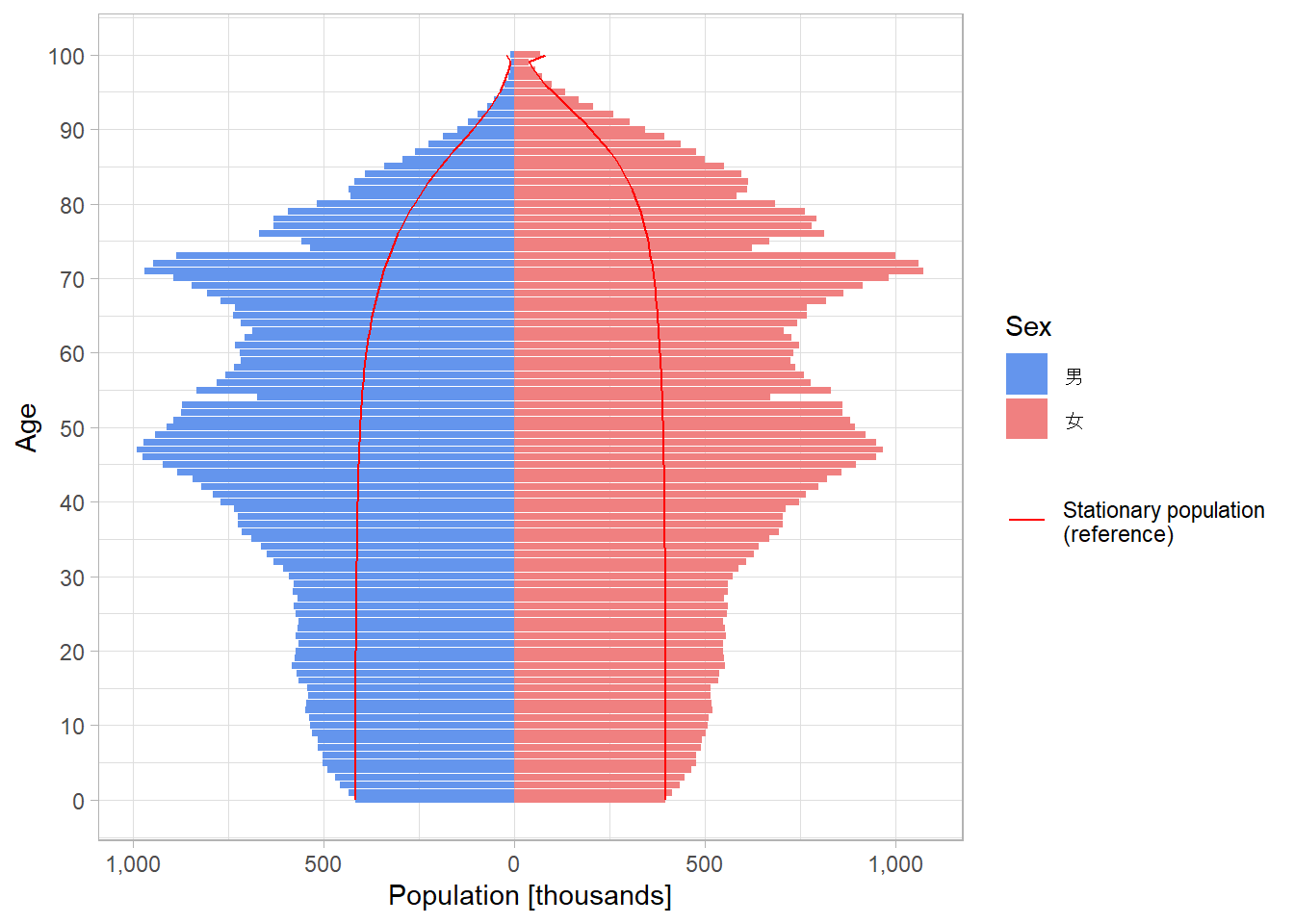
From the 2020 population pyramid, we can see population peaks in the early 70s and late 40s. These correspond to the generations known as the “dankai generation” (baby boomers) and the “dankai junior generation” (their children), respectively11. On the other hand, the population of younger generations is far smaller than that of the dankai generation and dankai junior generation, which illustrates just how severe the recent decline in the birthrate has become.
Let’s quantify the generational “vote-value disparity” using the ratio of the census population to the stationary population (reference value) shown by the red line.
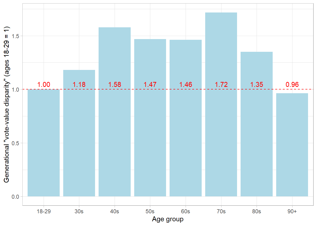
The graph below quantifies the generational “vote-value disparity,” in roughly 10-year intervals, for those aged 18 and over who are eligible to vote. Here, the “value of a vote” for those aged 18-29 is normalized to 1.
The graph shows that a single vote from those in their 40s to 60s is worth roughly 1.5 times that of a vote from those aged 18-29, and a single vote from those in their 70s is worth roughly 1.7 times that of a vote from those aged 18-29. We also found that the value of a vote for those in their 30s and those aged 80 and over — generations that don’t correspond to the “dankai generation” or “dankai junior generation” — is lower than for those in their 40s-60s and 70s (though this may be a result of the characteristics of the life table).
```{.r .cell-code code-fold=“true” code-summary=“Quantifying the generational”vote-value disparity”“} vote_disparity <- pop_2020 |> left_join(static_pop_2020 |> rename(static_pop = pop), by = join_by(sex, age)) |> filter(age >= 18) |> mutate(ageclass = case_when(between(age, 18, 29) ~”18-29”, between(age, 30, 39) ~ “30s”, between(age, 40, 49) ~ “40s”, between(age, 50, 59) ~ “50s”, between(age, 60, 69) ~ “60s”, between(age, 70, 79) ~ “70s”, between(age, 80, 89) ~ “80s”, 90 <= age ~ “90+”)) |> summarise(across(c(pop, static_pop), sum), .by = ageclass) |> mutate(vote_disparity = pop / static_pop, .keep = “unused”)
vote_disparity <- vote_disparity |> bind_cols(vote_disparity |> filter(ageclass == “18-29”) |> select(!ageclass) |> rename(vote_disparity_18to29 = vote_disparity)) |> mutate(vote_disparity = vote_disparity / vote_disparity_18to29, .keep = “unused”)
plot_vote_disparity <- vote_disparity |> ggplot(aes(ageclass, vote_disparity)) + geom_col(fill = “lightblue”) + geom_text(aes(label = scales::label_comma(accuracy = 1e-2)(vote_disparity)), y = 1, vjust = -0.5, color = “red”) + geom_hline(yintercept = 1, color = “red”, linetype = “dashed”) + scale_x_discrete(“Age group”) + scale_y_continuous(“Generational "vote-value disparity" (ages 18-29 = 1)”)
ggsave(“quantify-vote-disparity-between-generations/plot_vote_disparity.png”, plot = plot_vote_disparity)
plot_vote_disparity ```
Using the open data of the Population Census and the Life Tables, I quantified the generational “vote-value disparity.”
In fact, it’s said that low voter turnout among young people is also a major factor behind the generational “vote-value disparity.” Going forward, it will likely be necessary to deepen the discussion around the generational “vote-value disparity” while also proposing more appealing policies that raise voter turnout among the young.
The 20th Unified Local Elections, which determine local government assembly members and heads, were held on Sunday, April 9, 2023, and Sunday, April 23, 2023.↩︎
House of Councillors election: “vote-value disparity of up to 3.03 times” — Supreme Court Grand Bench to hear the case↩︎
This idea is similar to the notion mentioned above that, under the concentration of population in urban areas driven by Tokyo’s dominance, making the “value of a vote” completely equal could actually disadvantage rural areas.↩︎
Choosing Our Future (4): Measures Against the Declining Birthrate↩︎
The stationary population (reference value) shown by the red line represents how many of the men and women who were 0 years old in 2020 would still be alive at each age, under the assumption of a constant mortality rate.↩︎
The male-to-female ratio of the population at age 0 is approximately 105:100.↩︎
Seeing Japan’s Future Through the “Population Pyramid”!? — Aging and the “Dankai Generation,” the Declining Birthrate and the “Dankai Junior Generation”↩︎