Visualizing Municipal Mergers in Japan with R’s ggraph

Note: This article is translated from my Japanese article.

Yesterday, I introduced the jpcity package in this article. Internally, the jpcity package builds a network of Japan’s past municipal mergers (formally called haichi bungō, i.e., the establishment, abolition, and merger of municipalities) in order to map municipality codes across different points in time.

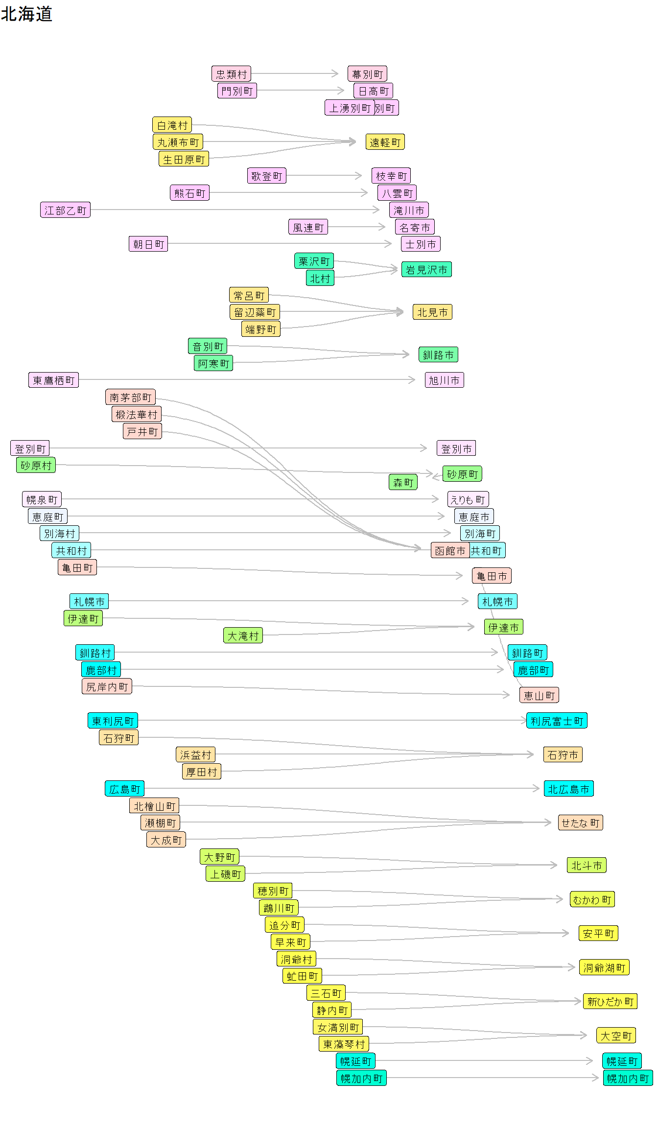
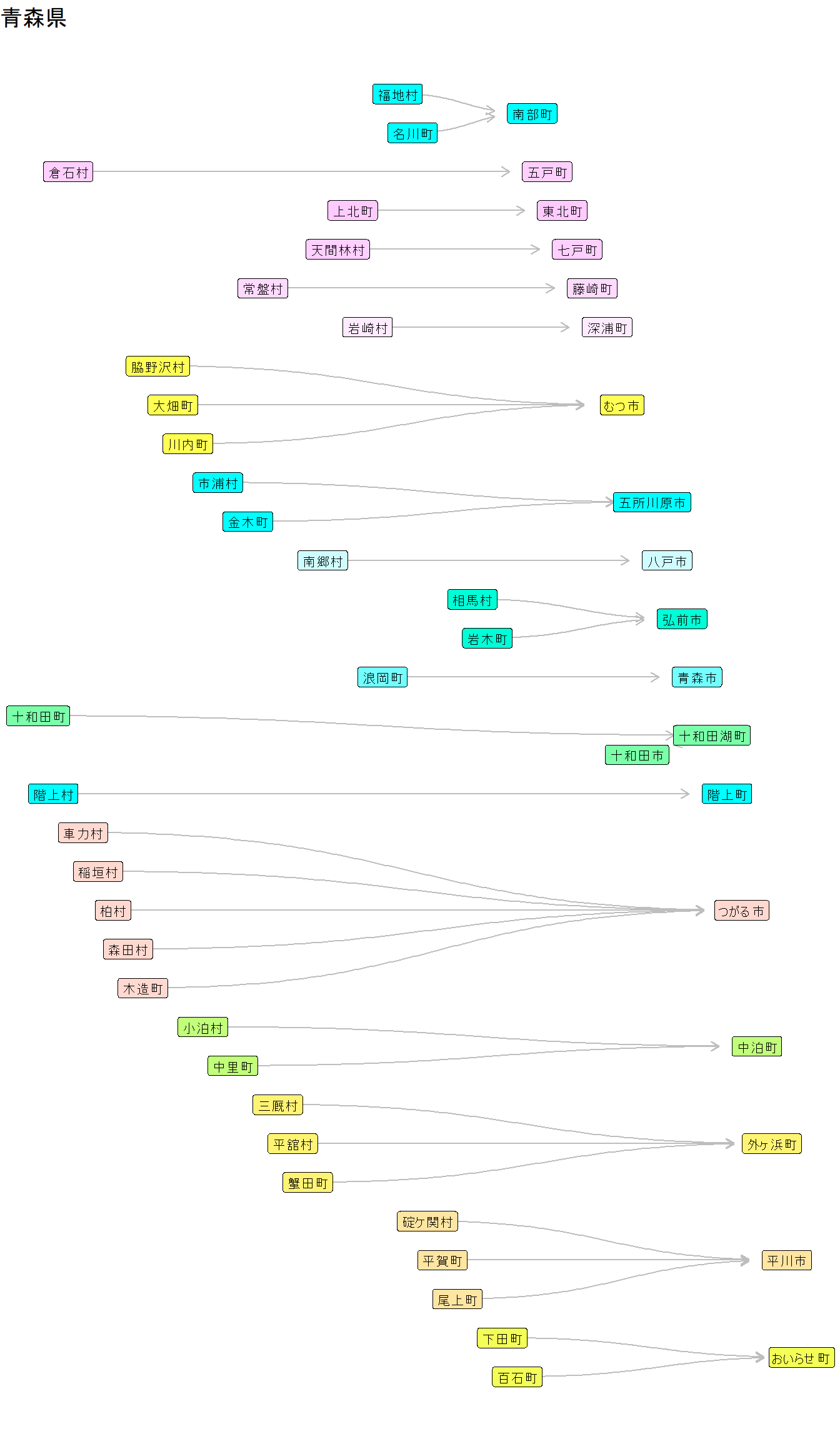
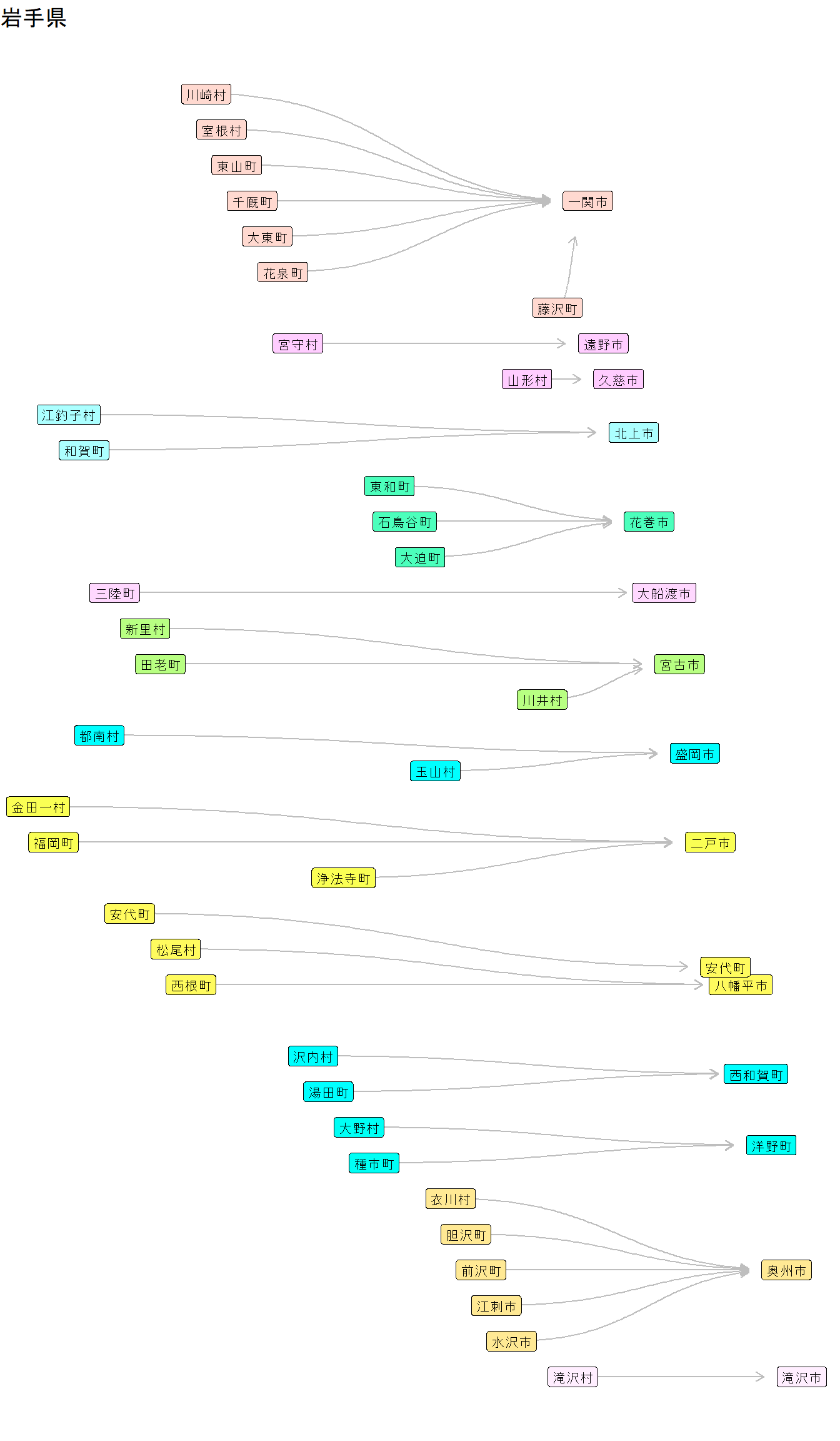
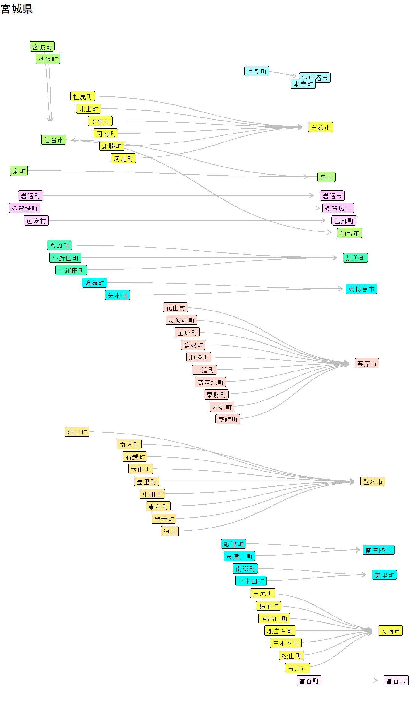
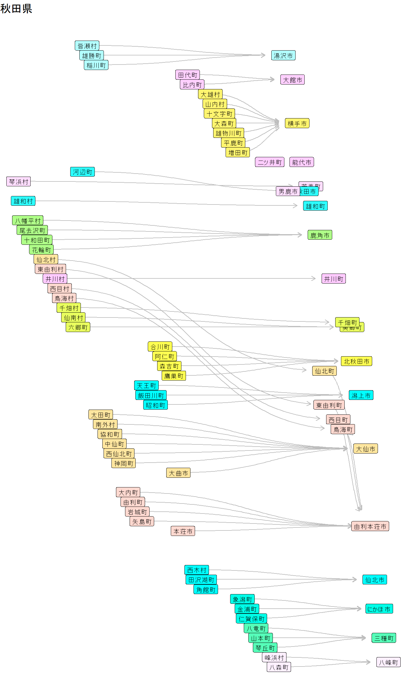
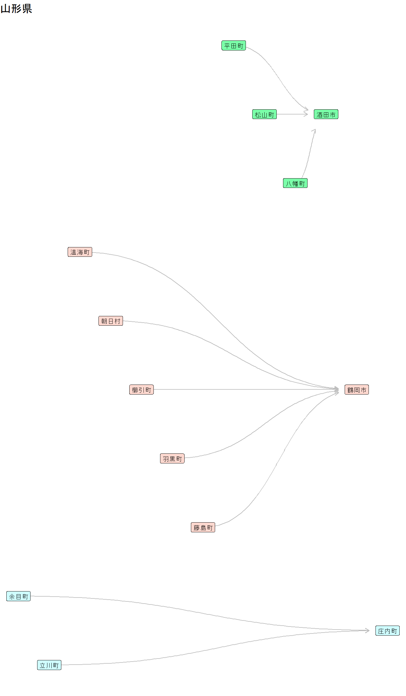
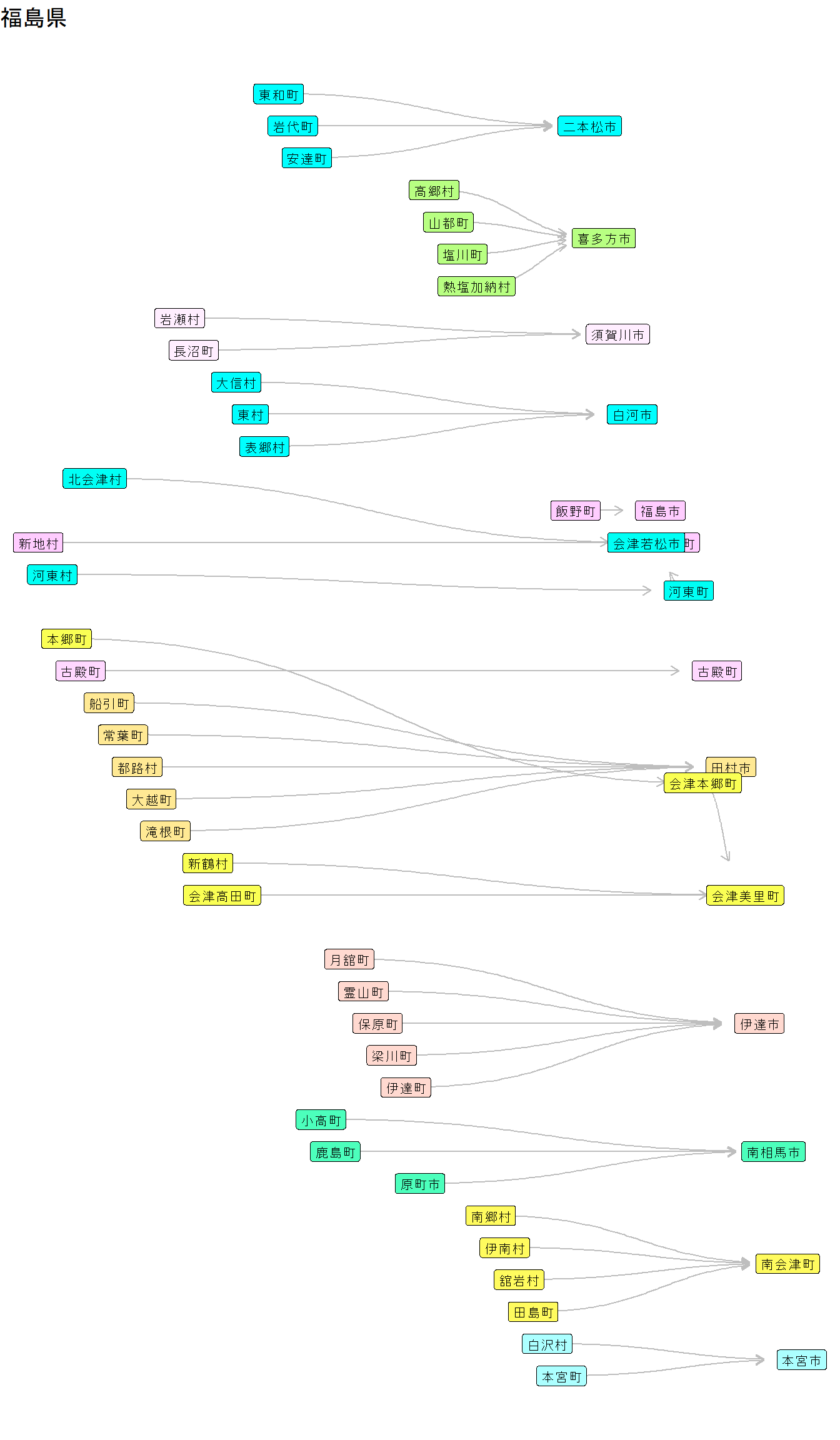
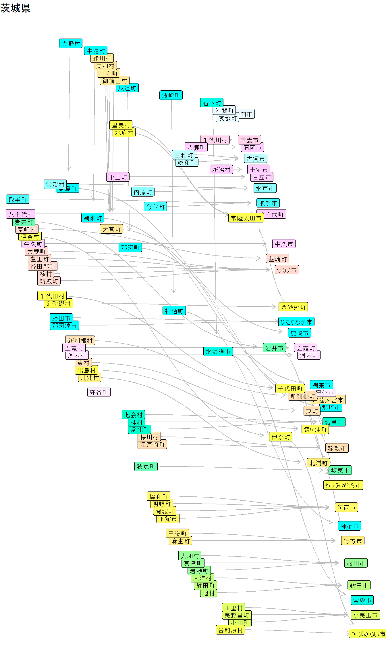
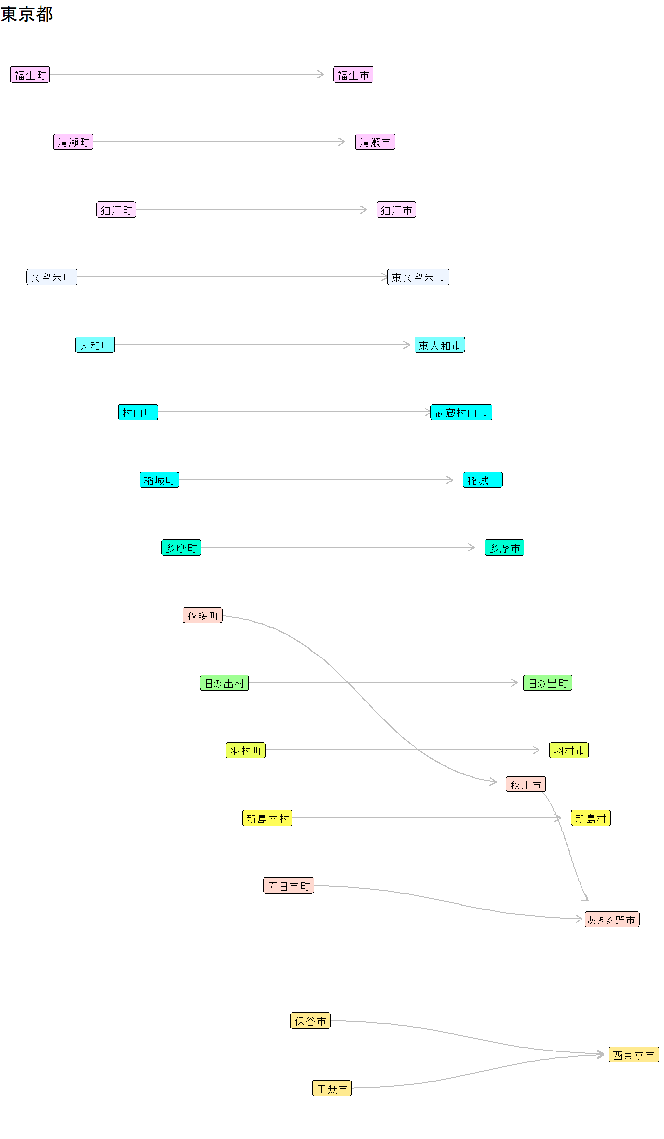
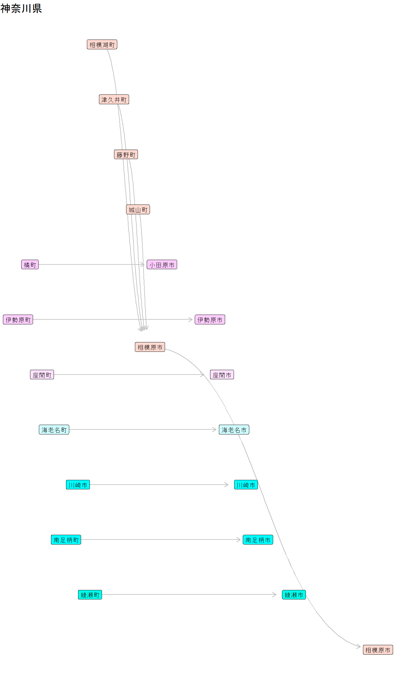
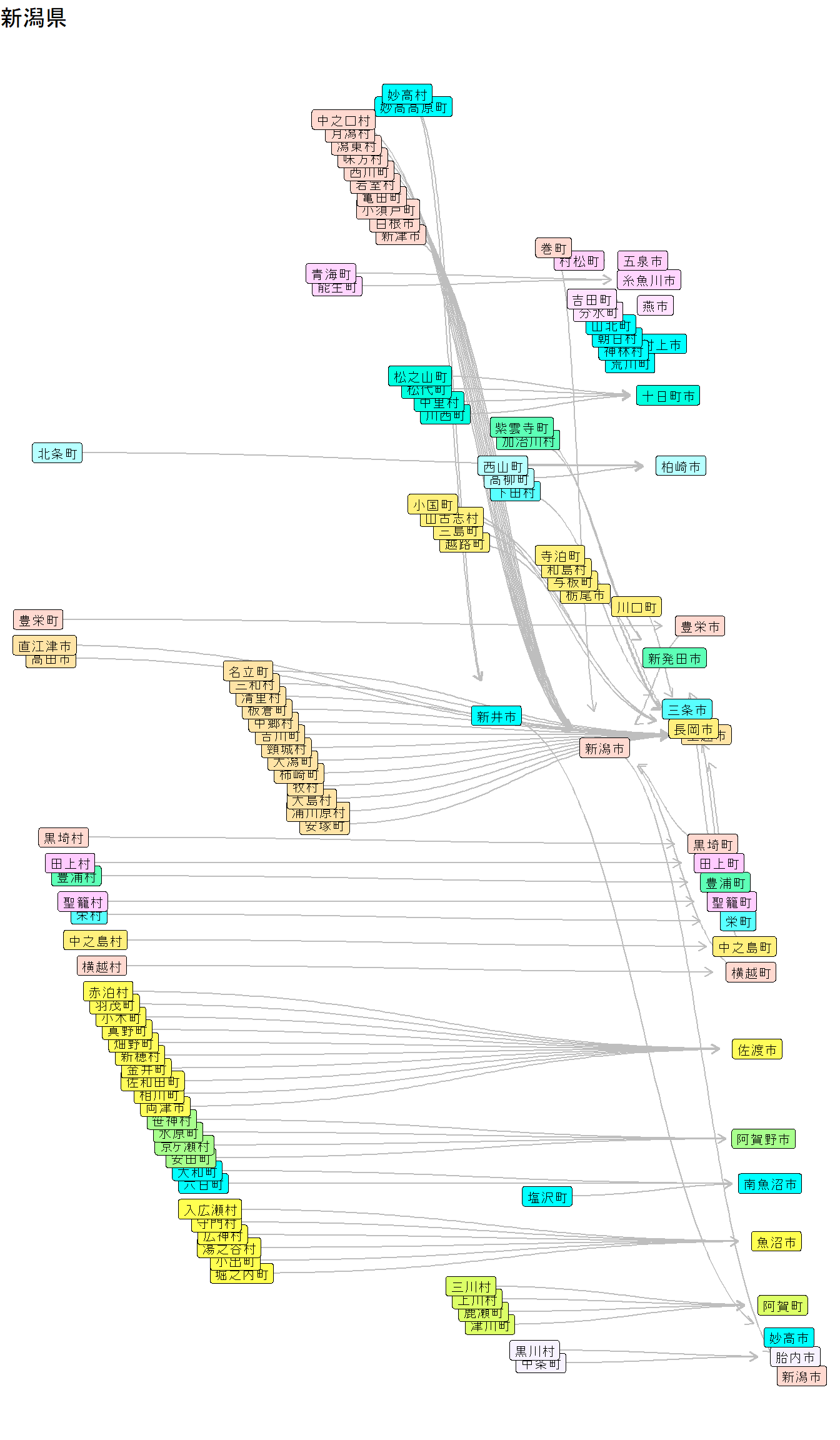
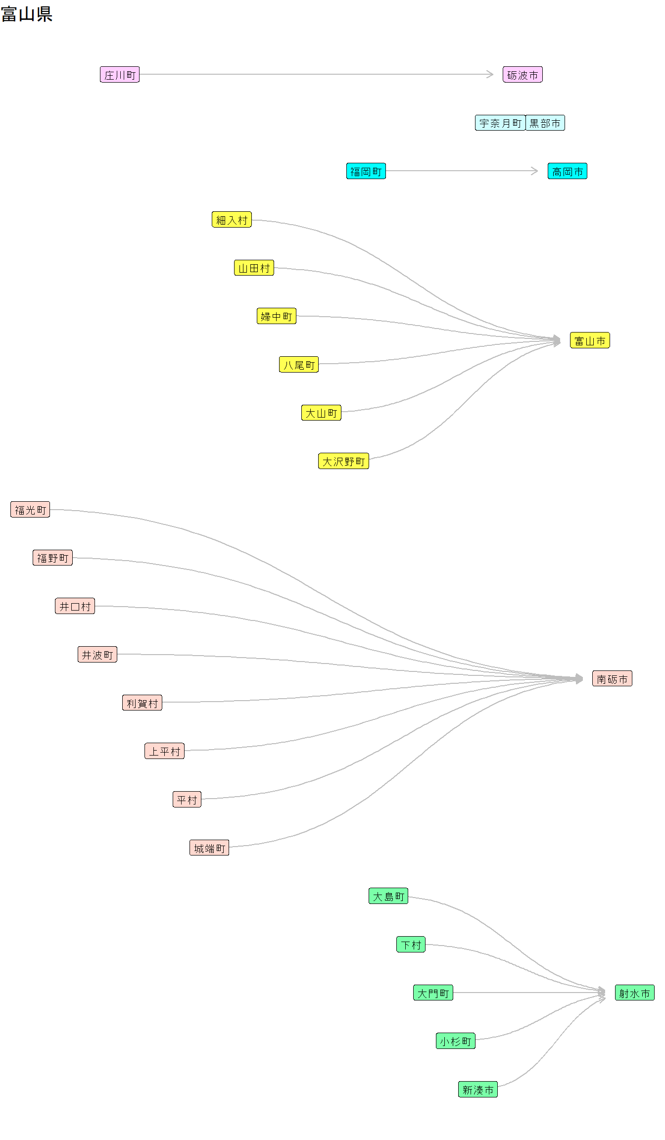
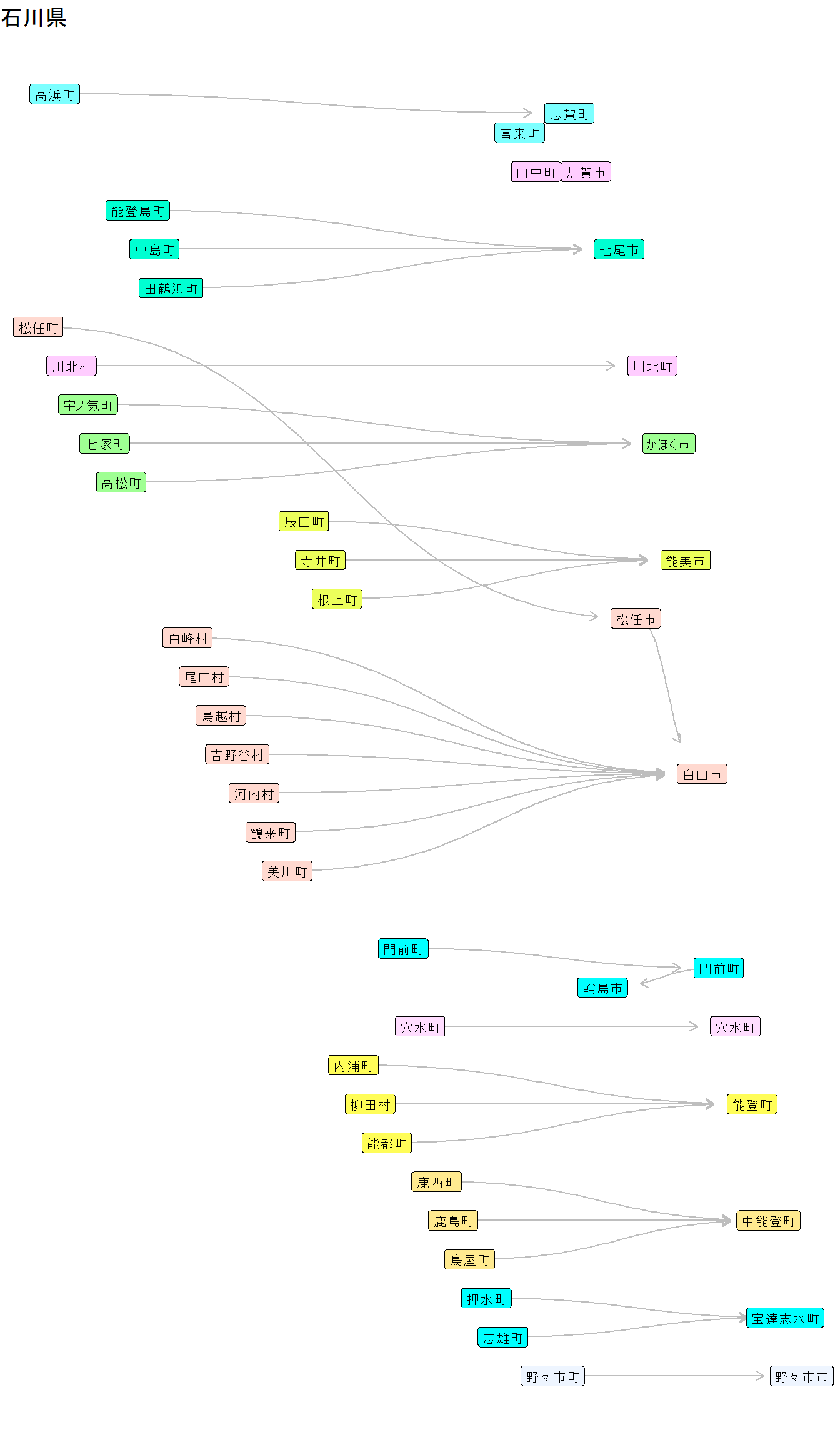
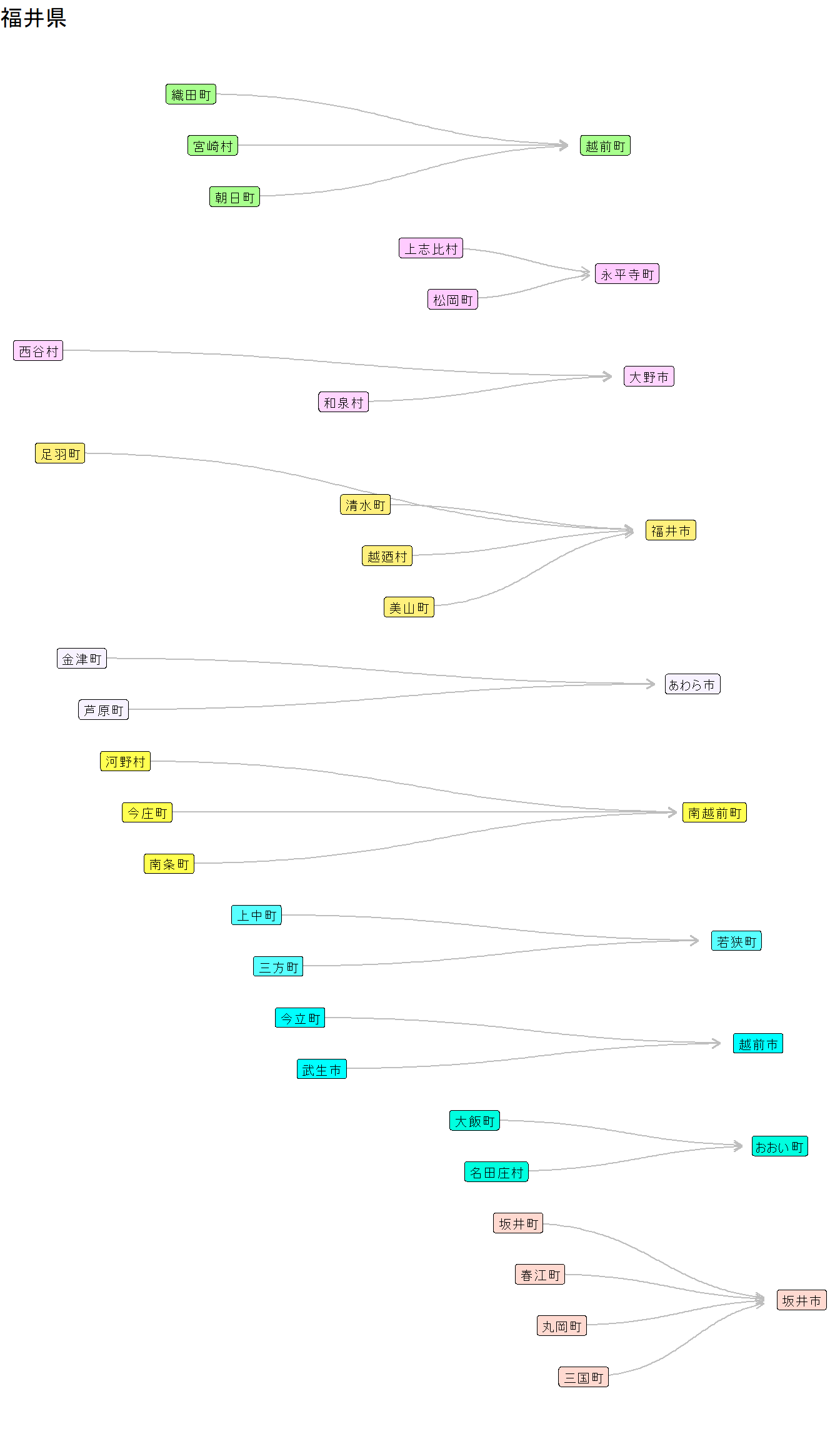
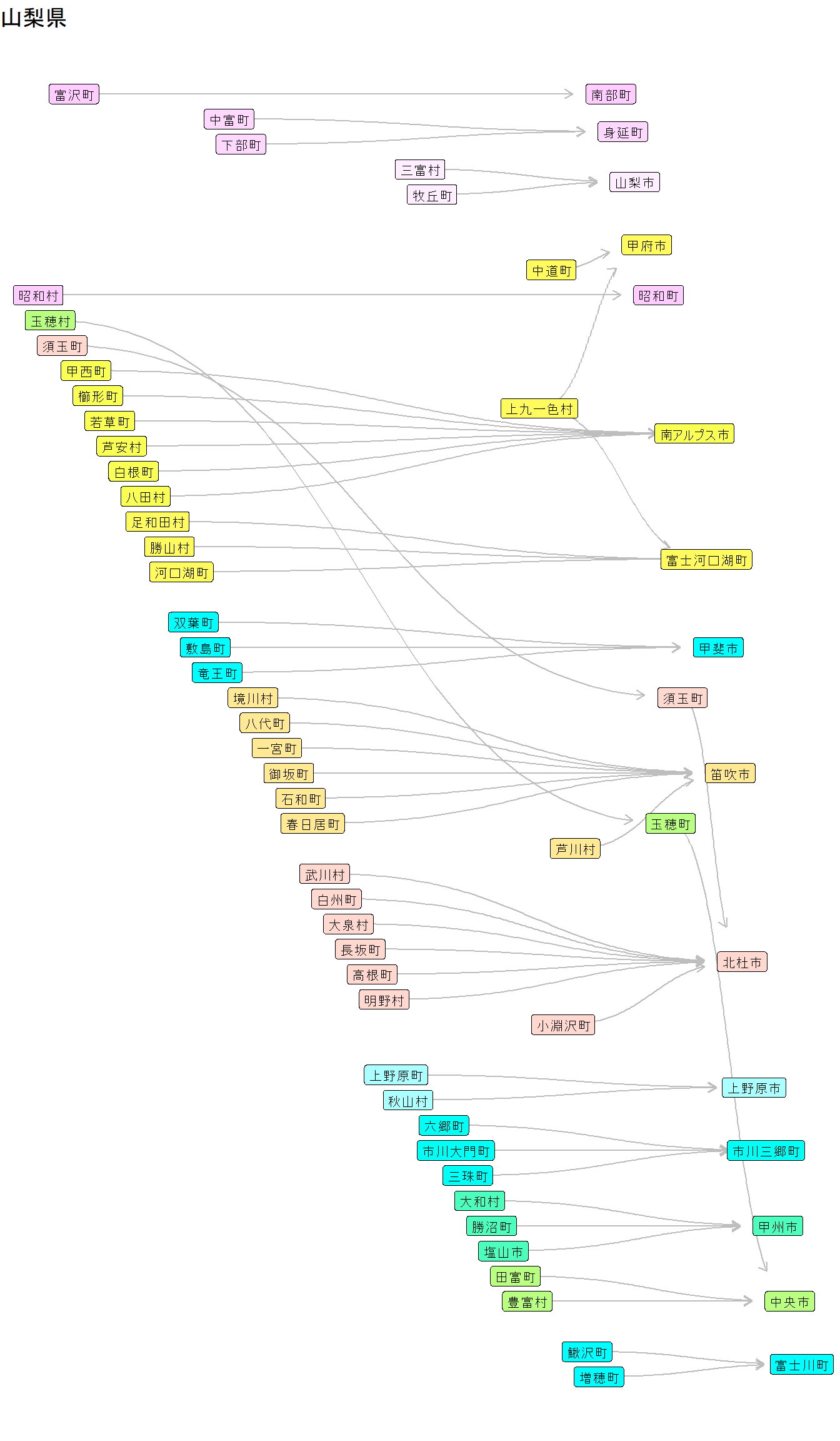
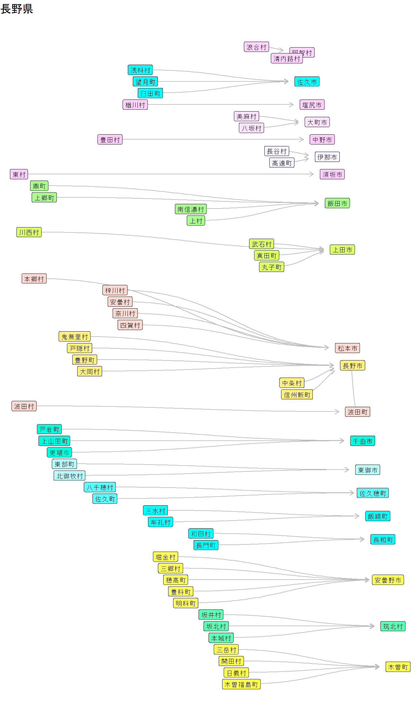
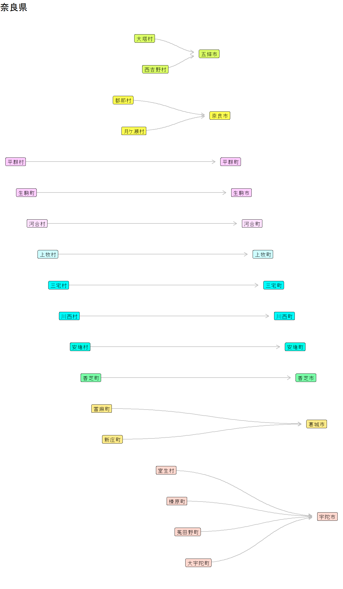
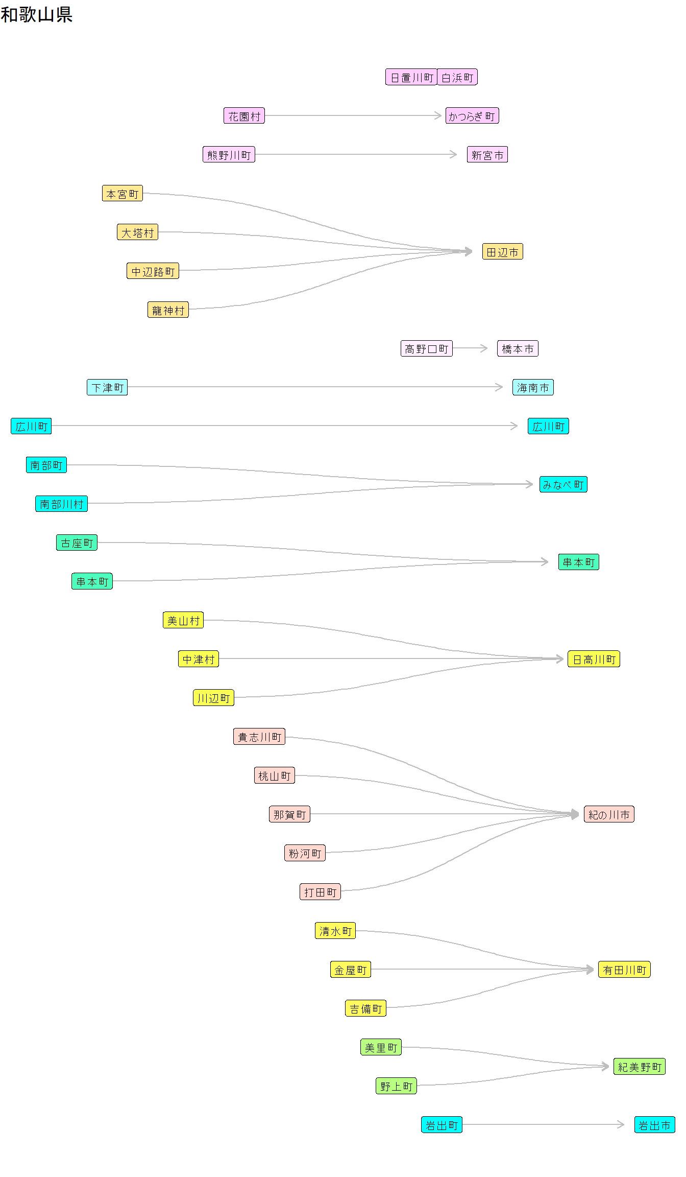
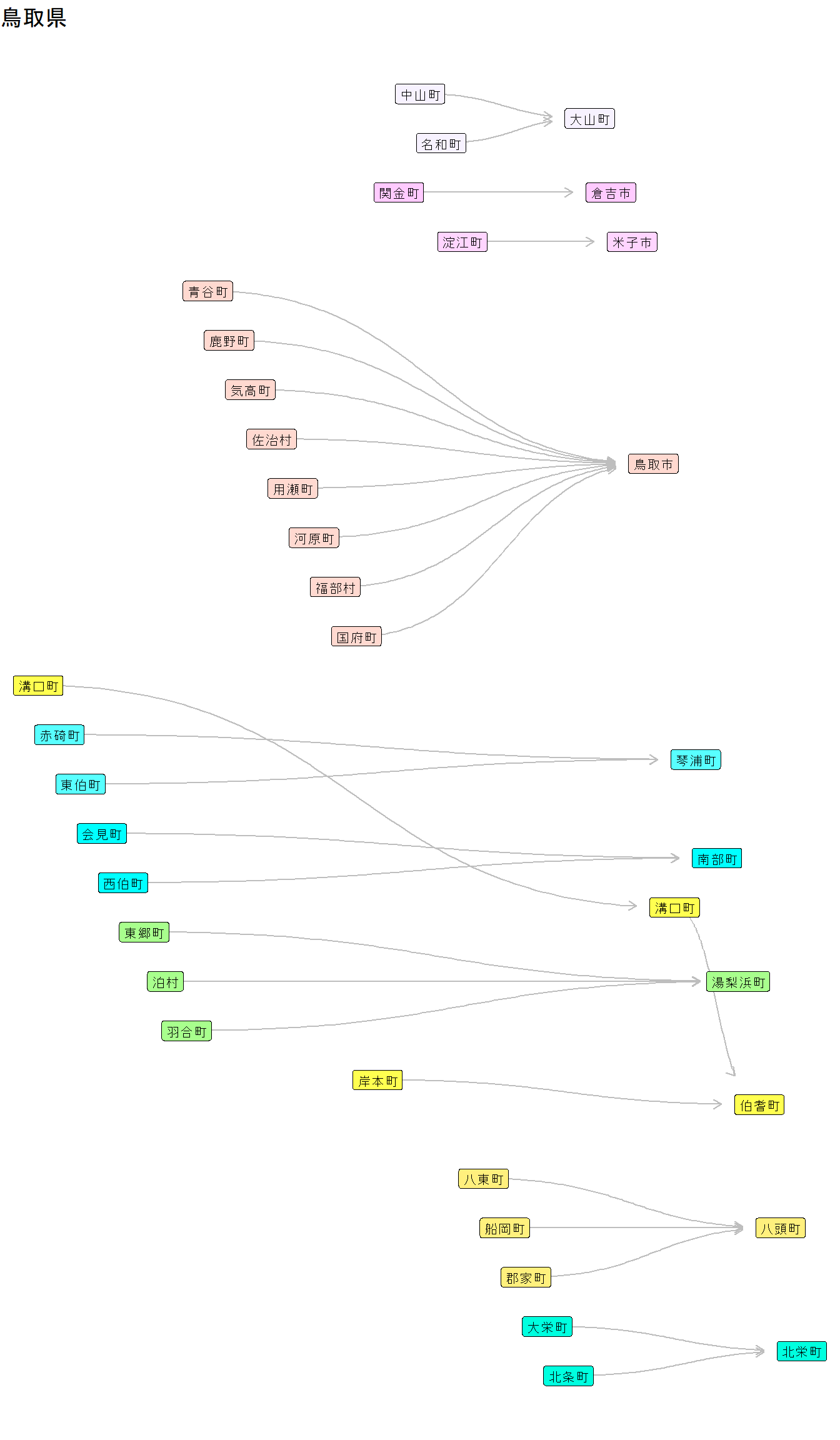
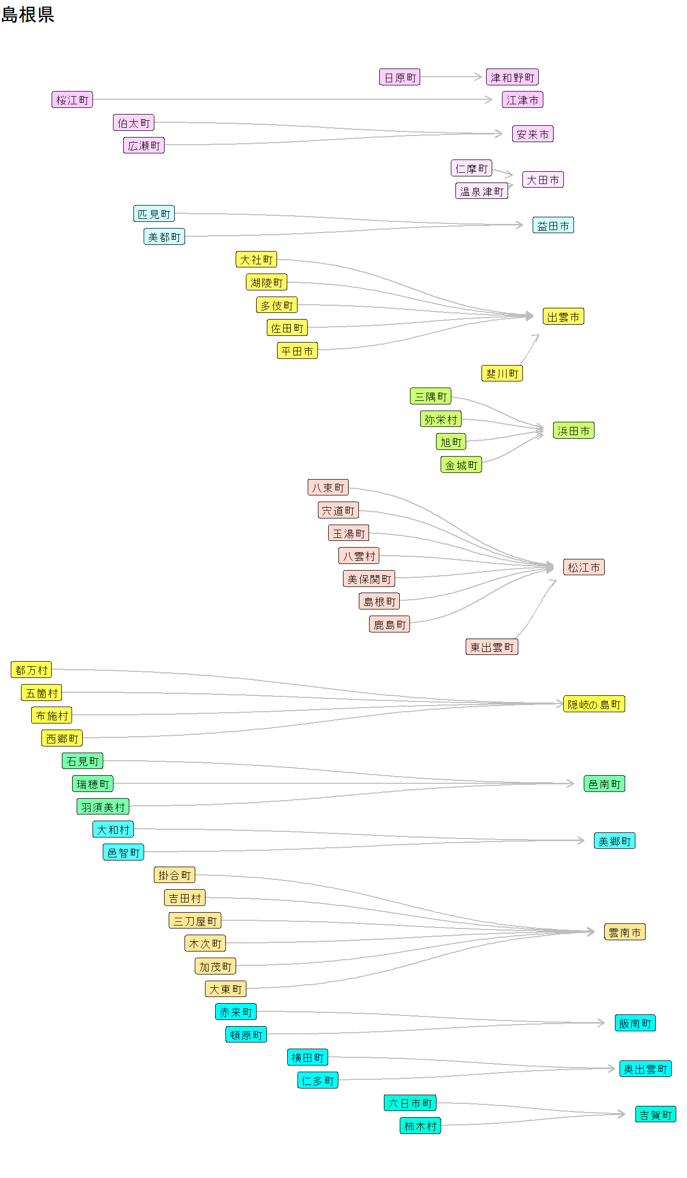
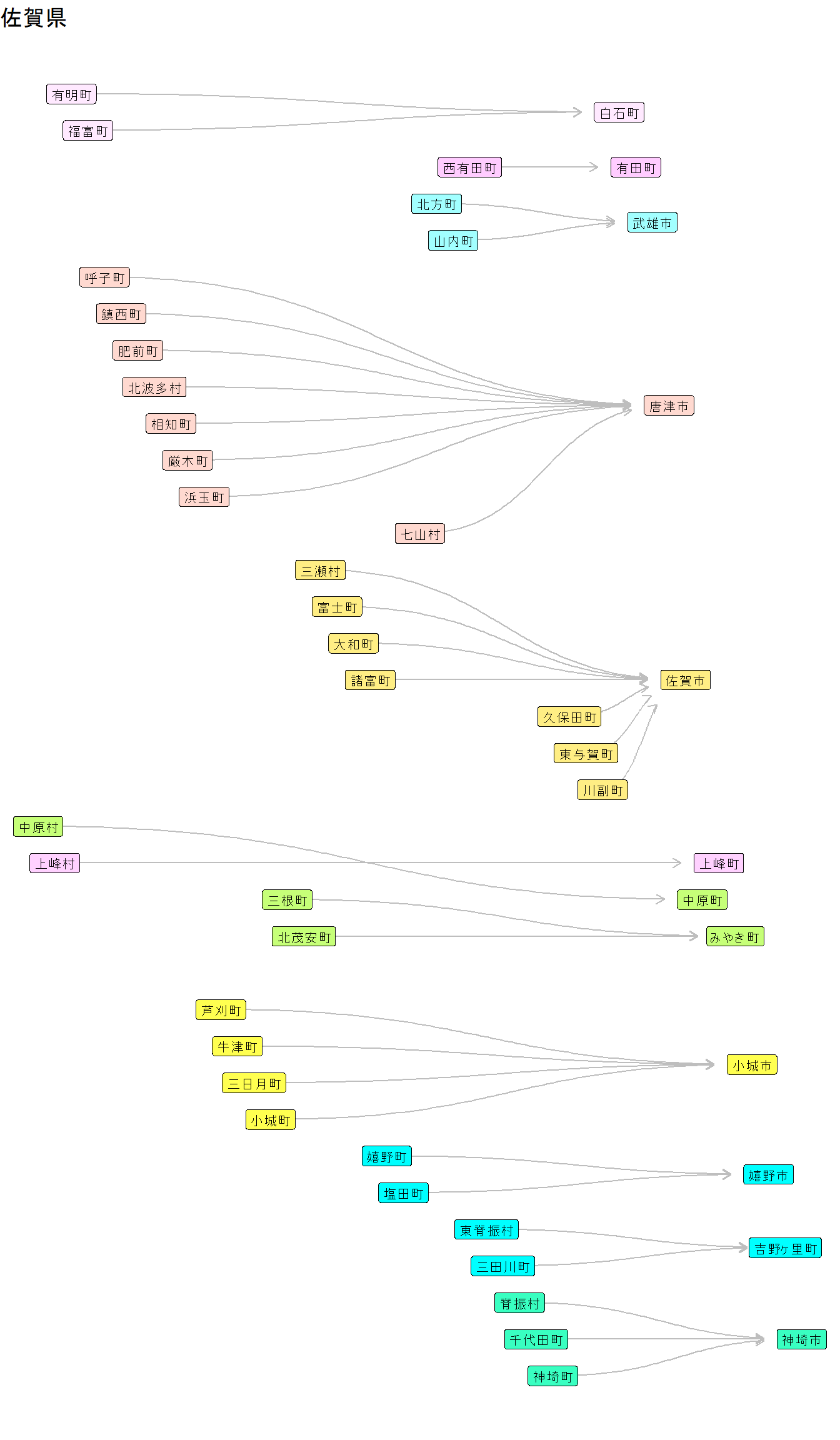
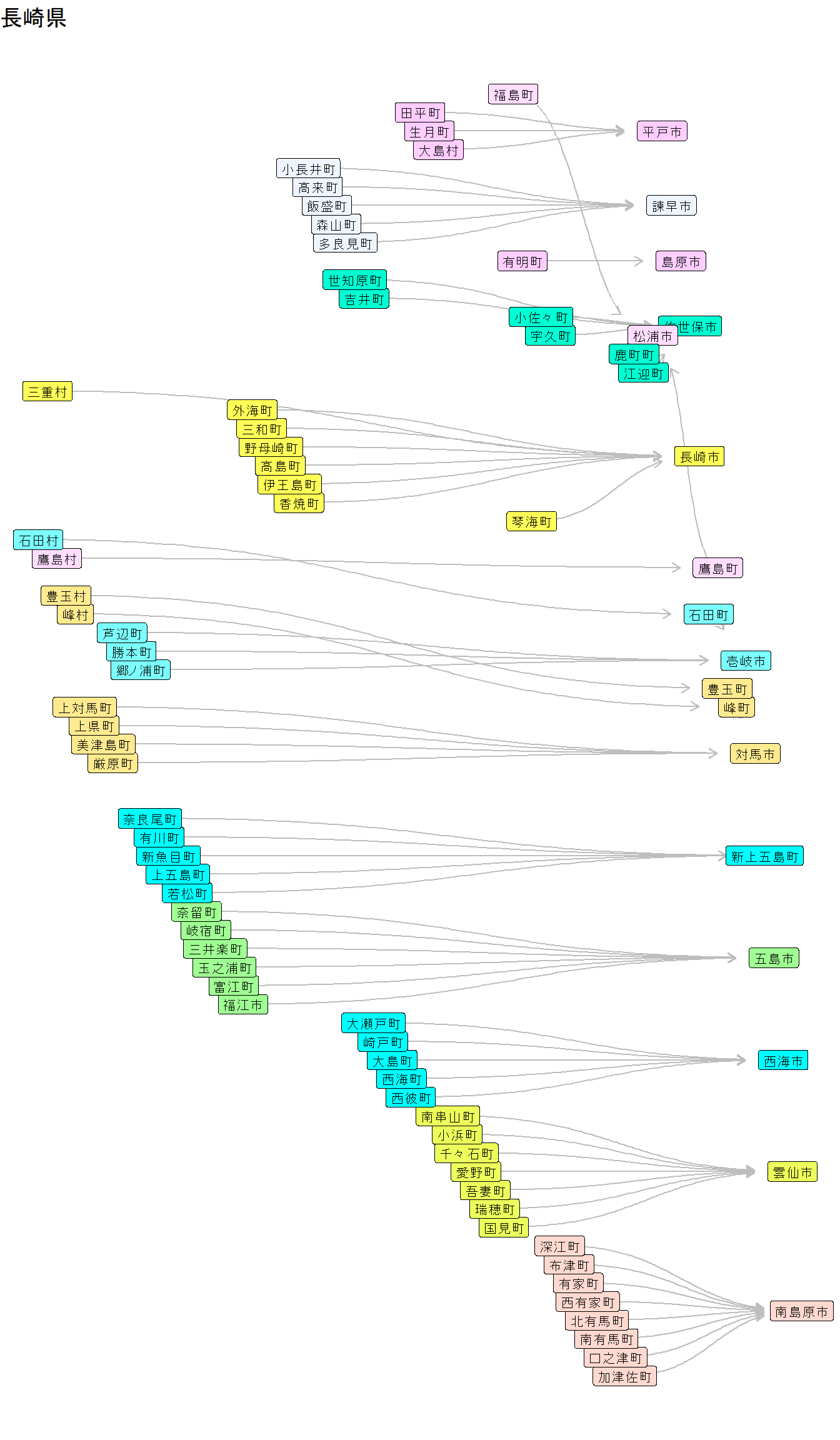
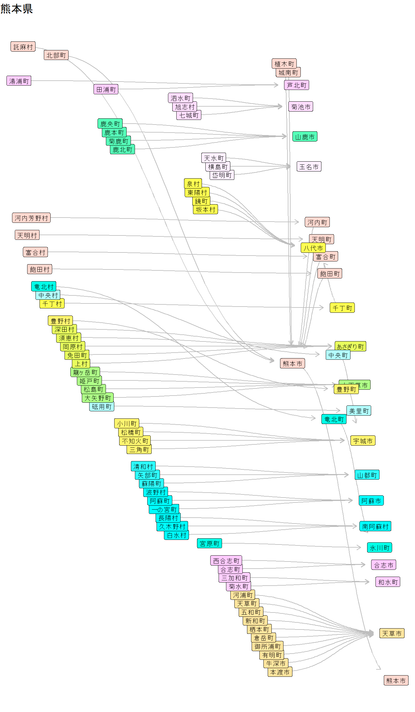
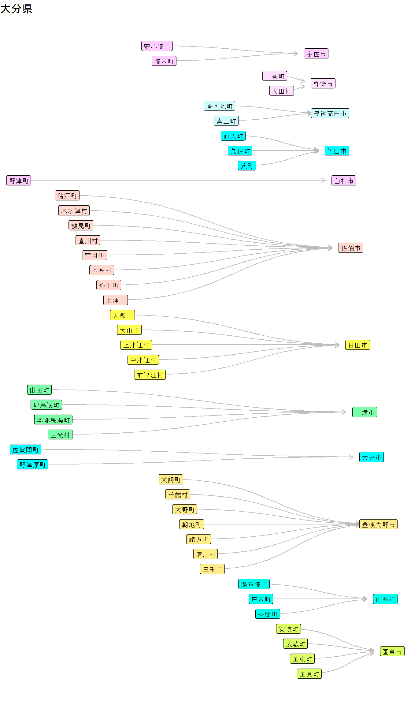
In this article, I’ll visualize the municipal merger network used internally by the jpcity package, following these guidelines:

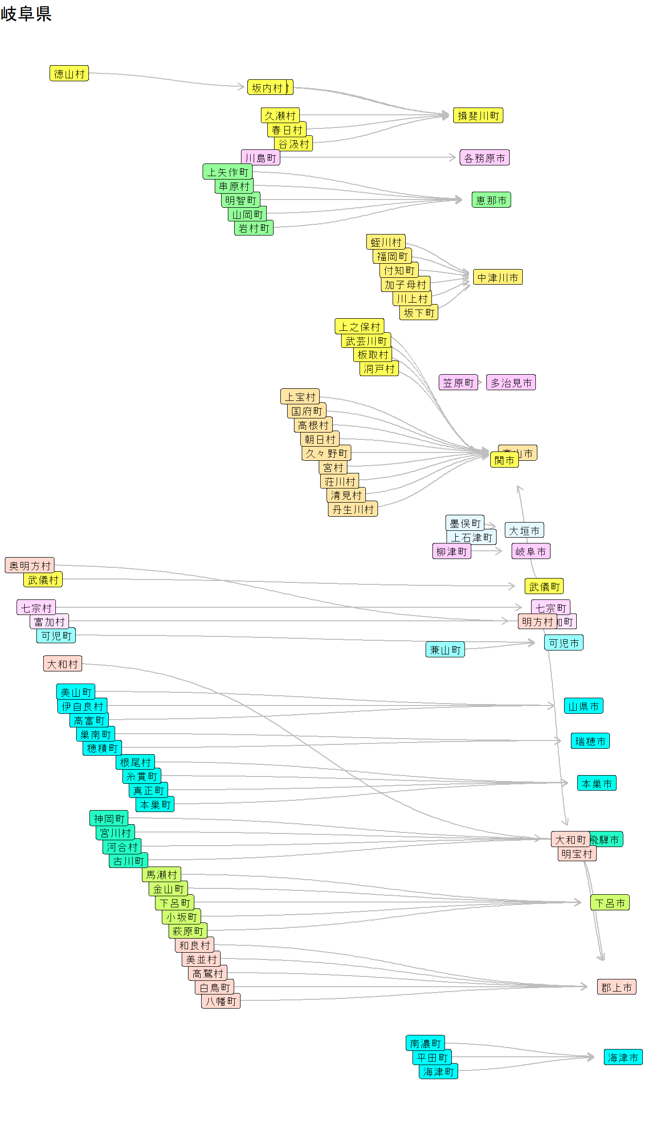
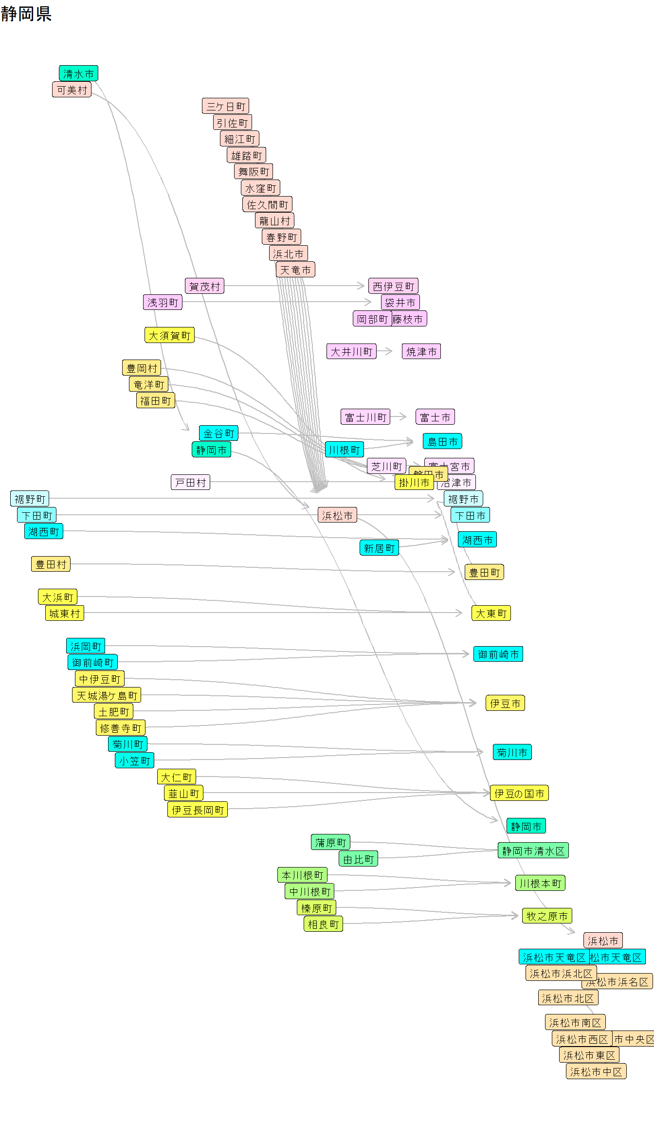
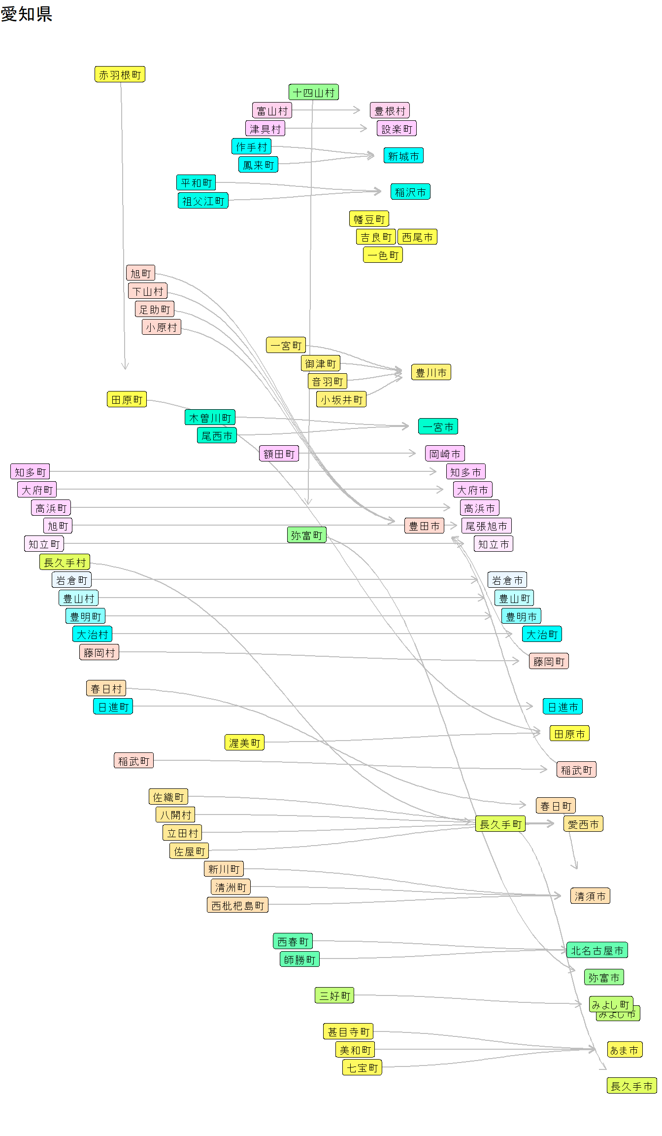
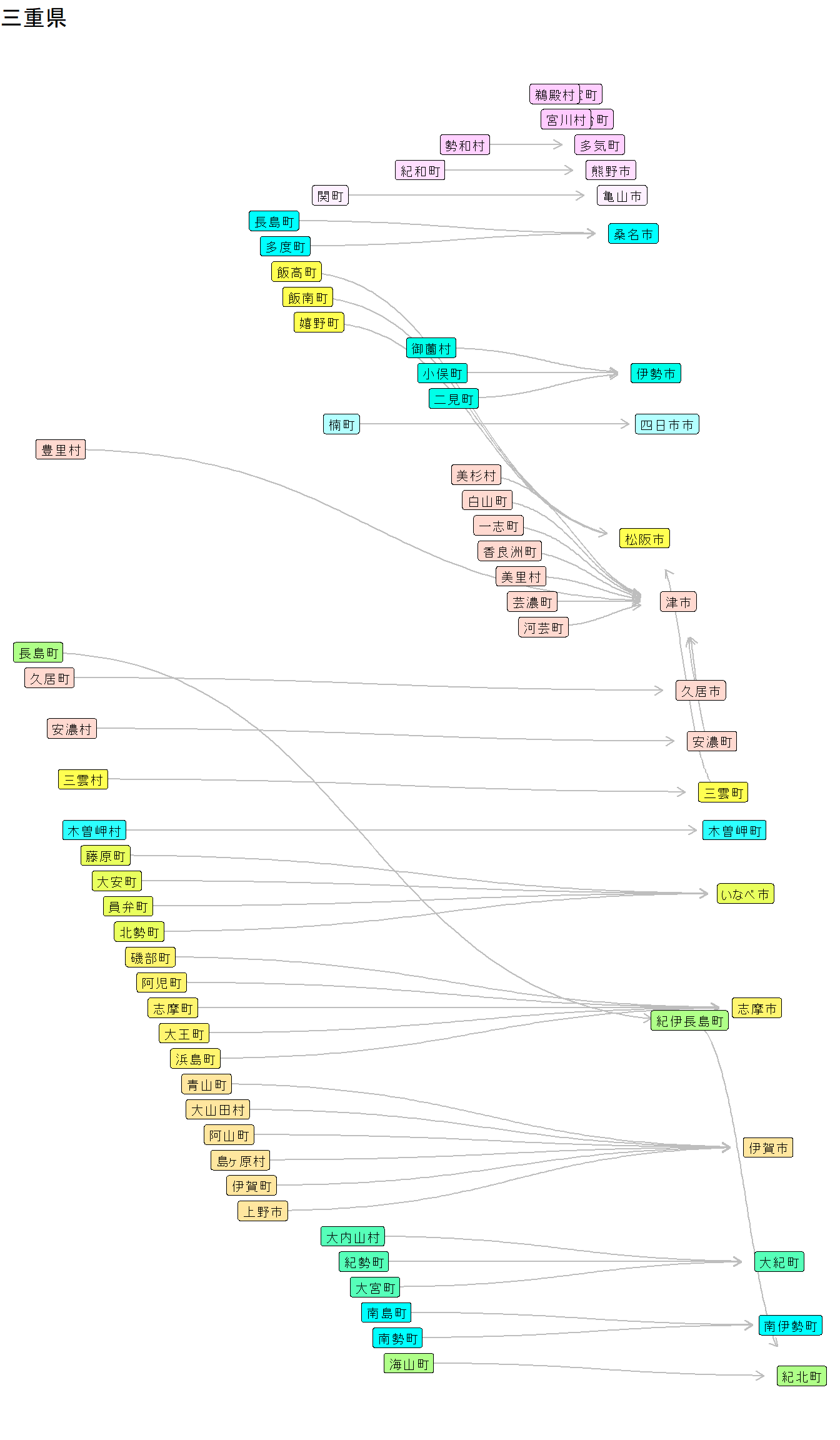
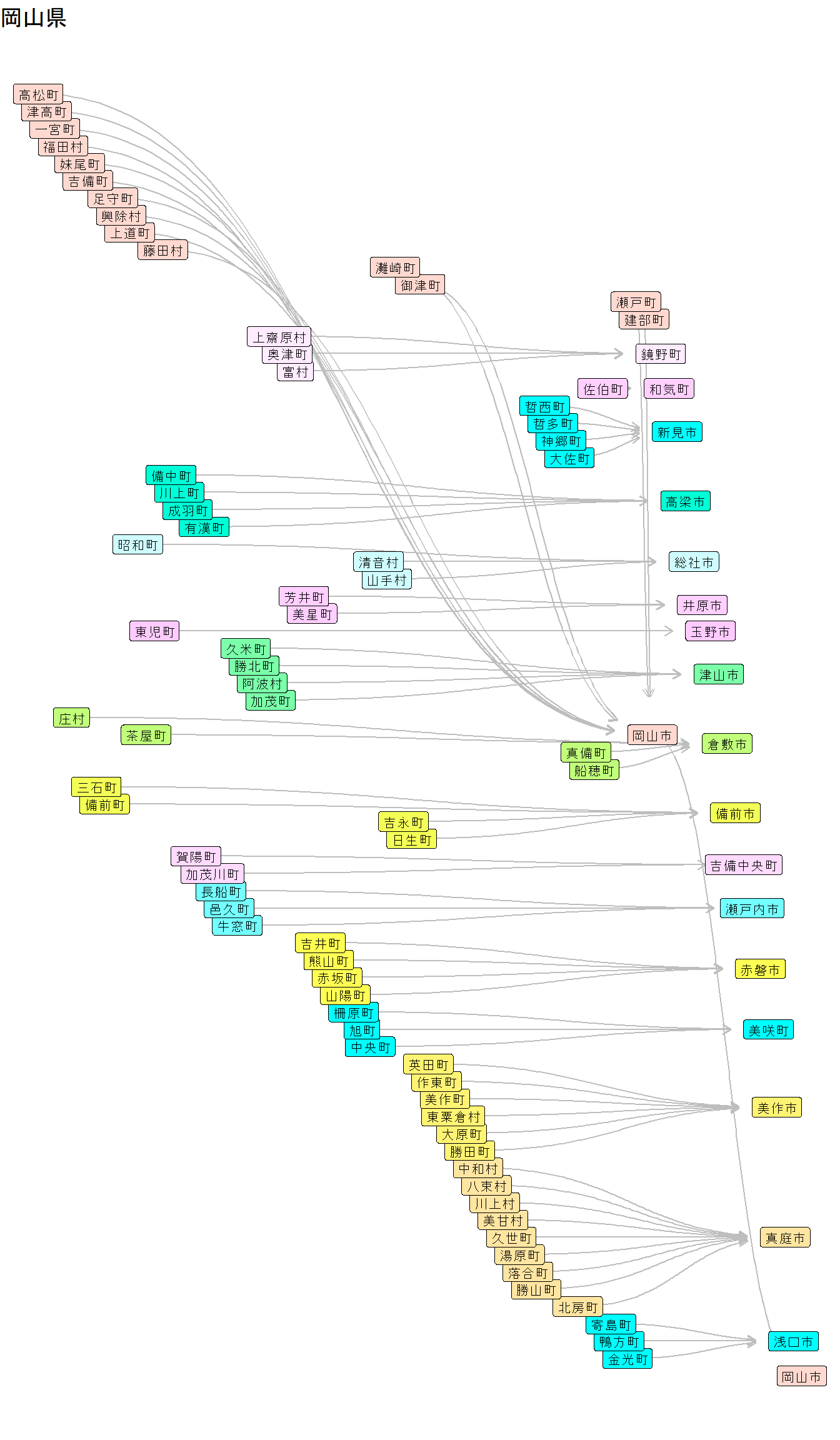
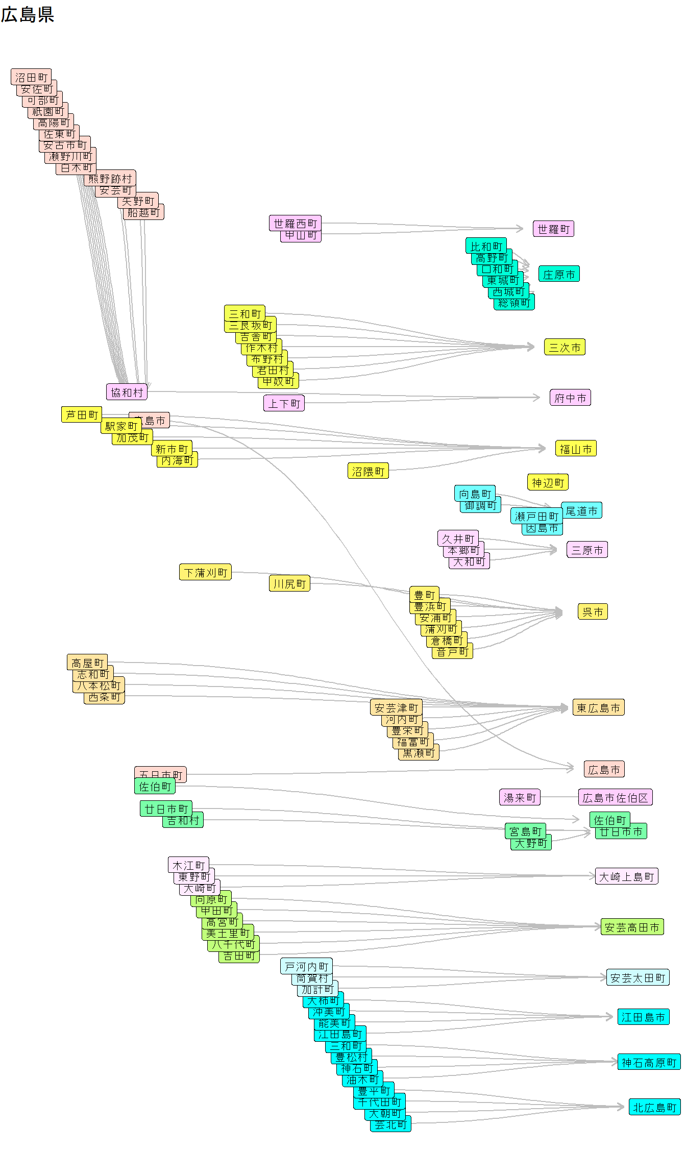
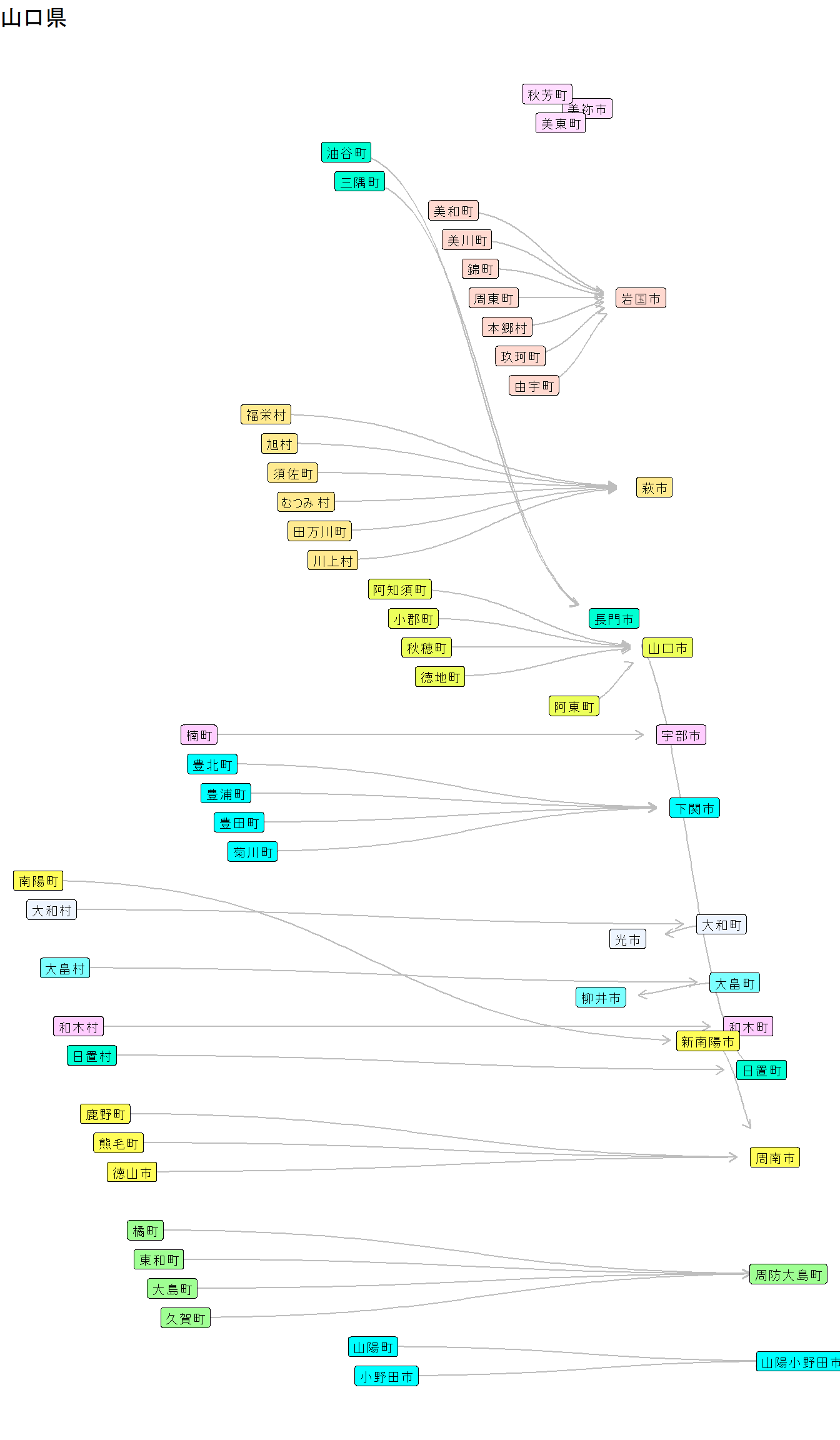
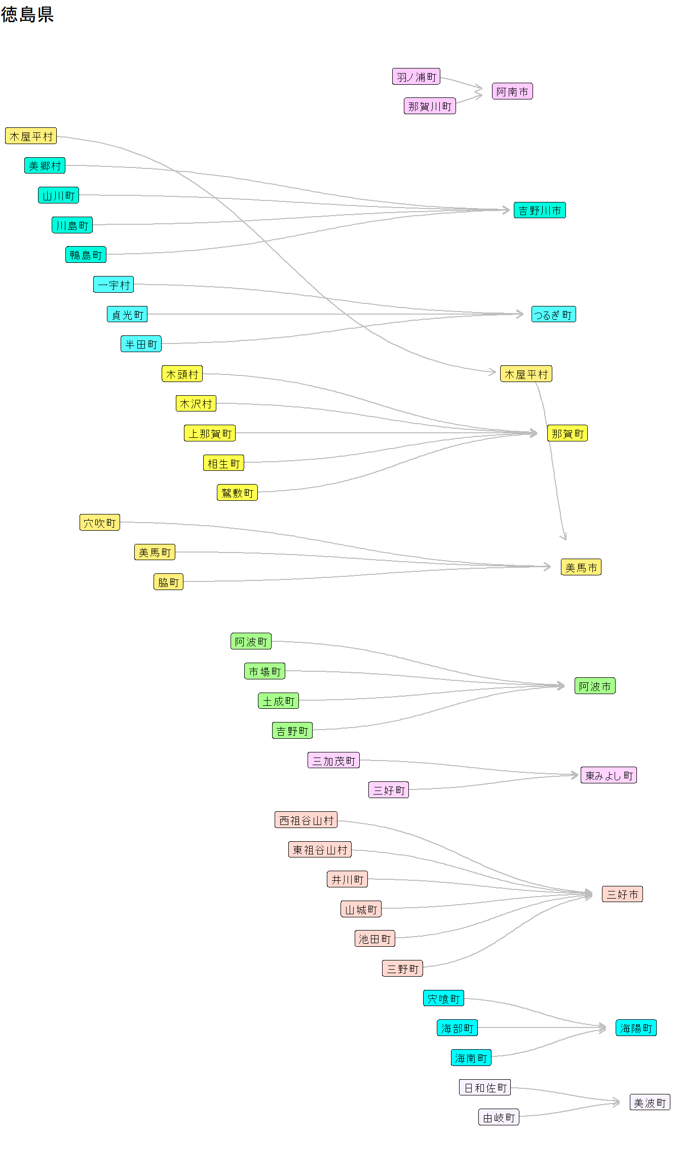
Visualize municipal mergers and city/town incorporations from April 1, 1970 to April 1, 2024, by prefecture
Node ordering does not take chronology into account (it’s possible to align positions with time, but this makes the graph harder to read)
Ward separations/splits are excluded

References

Let’s Smartly Format Municipal Data in R (aggregating municipal mergers, designated cities, etc.)

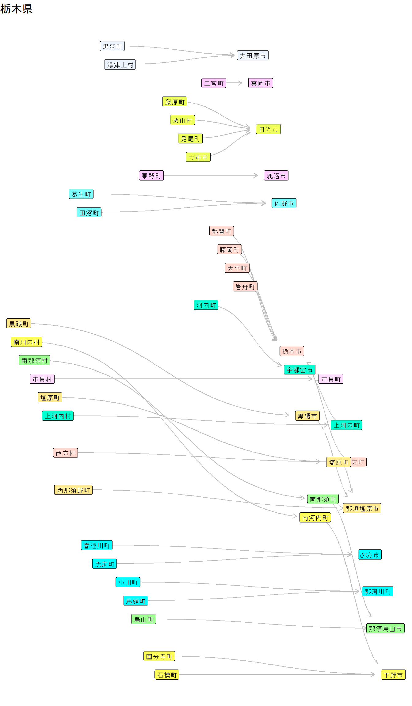
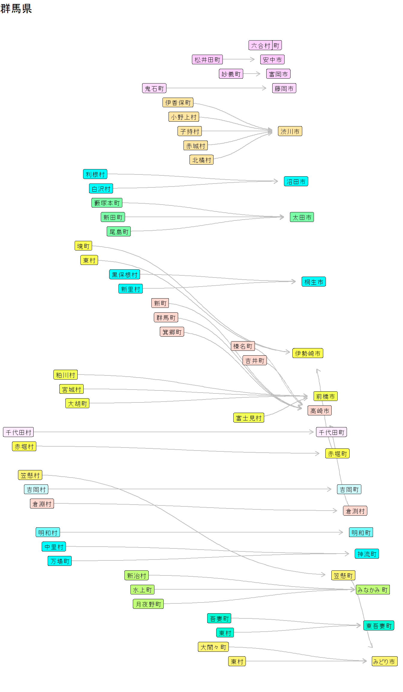
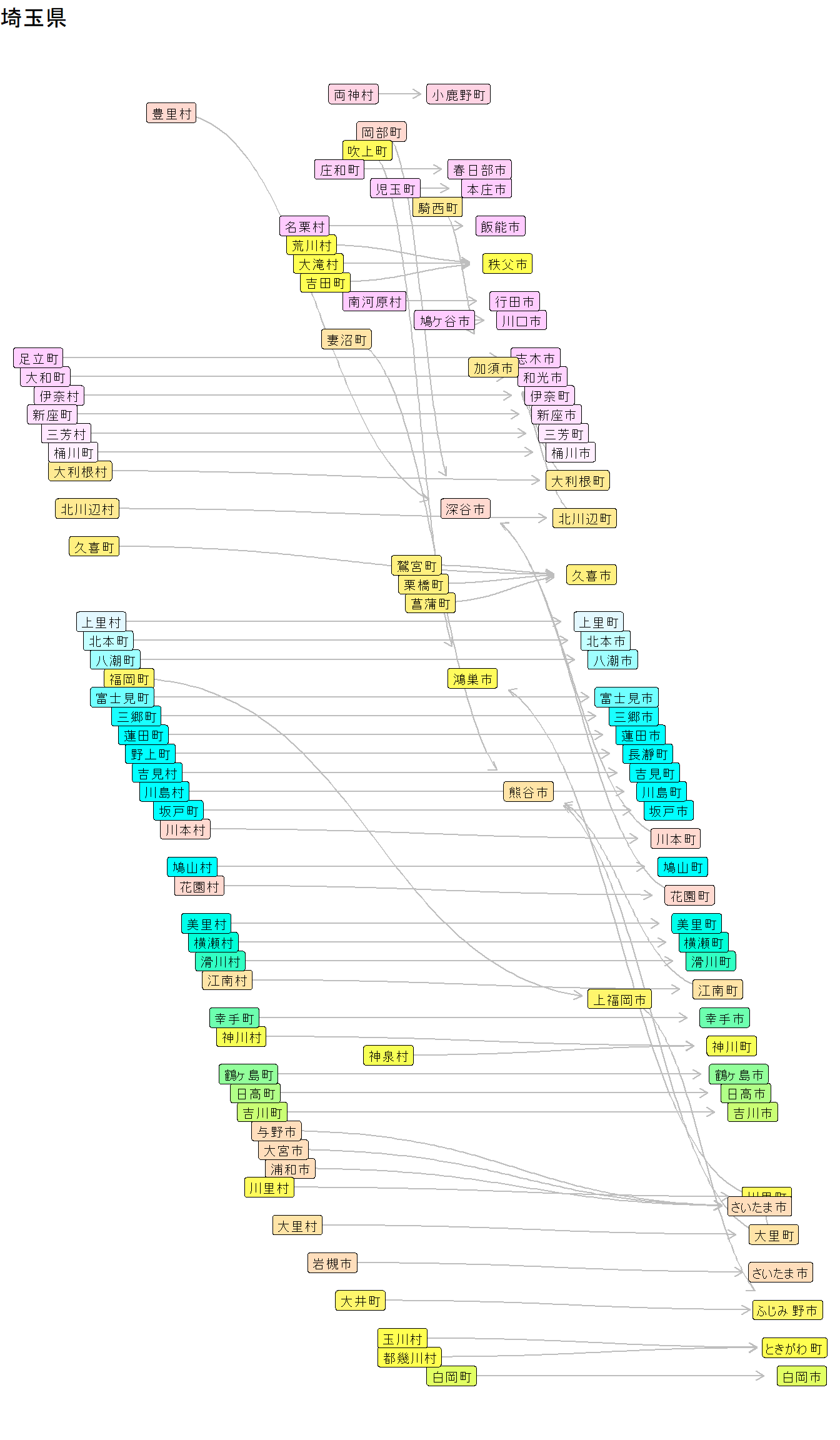
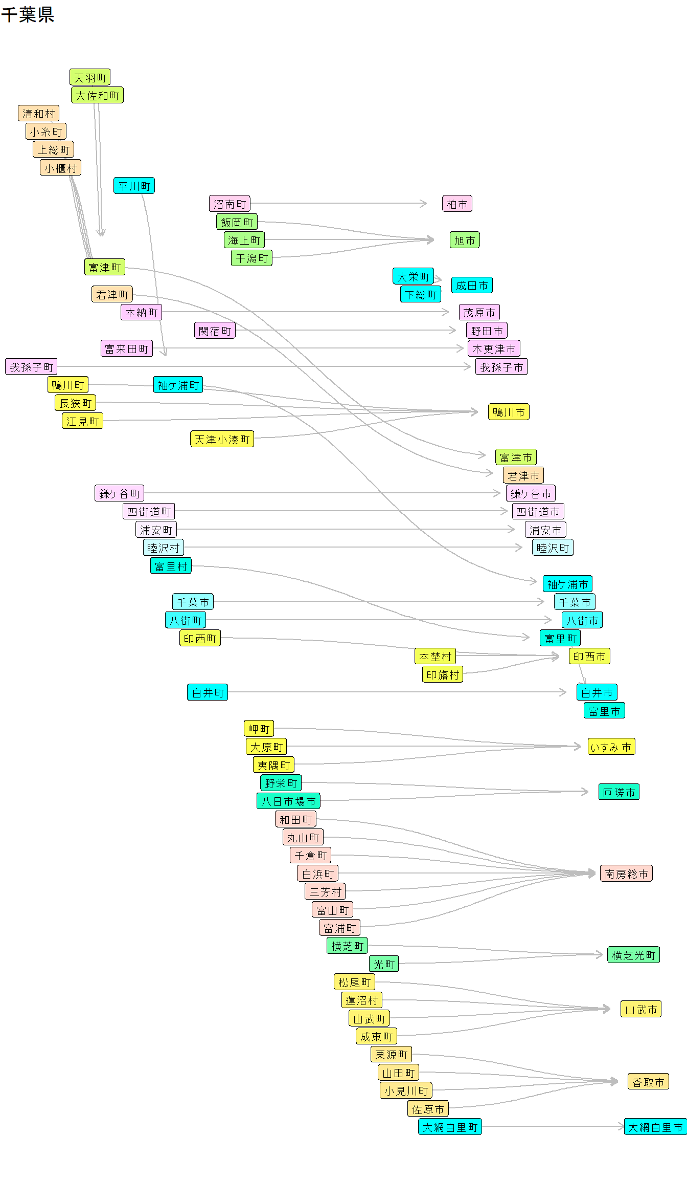
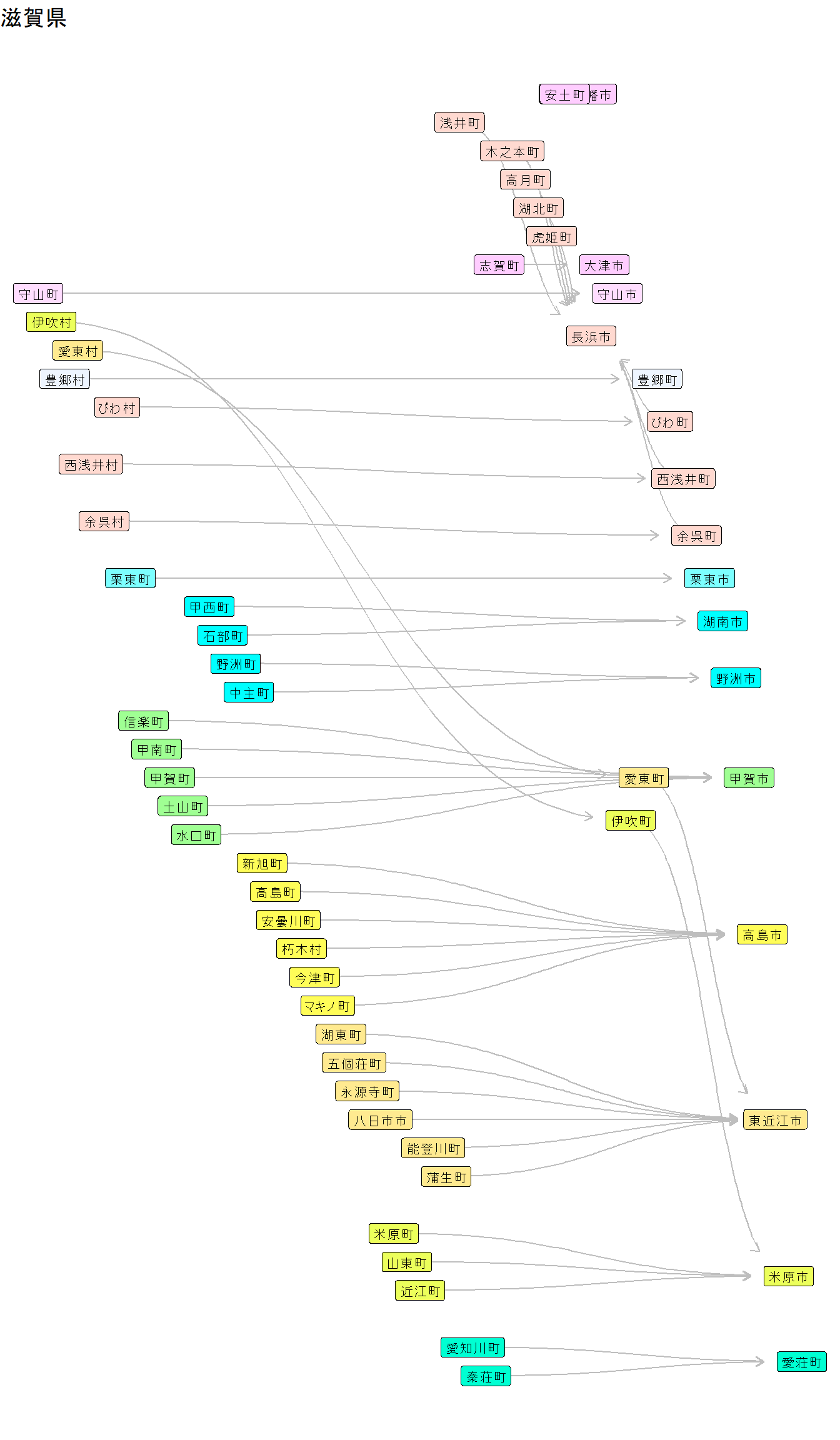
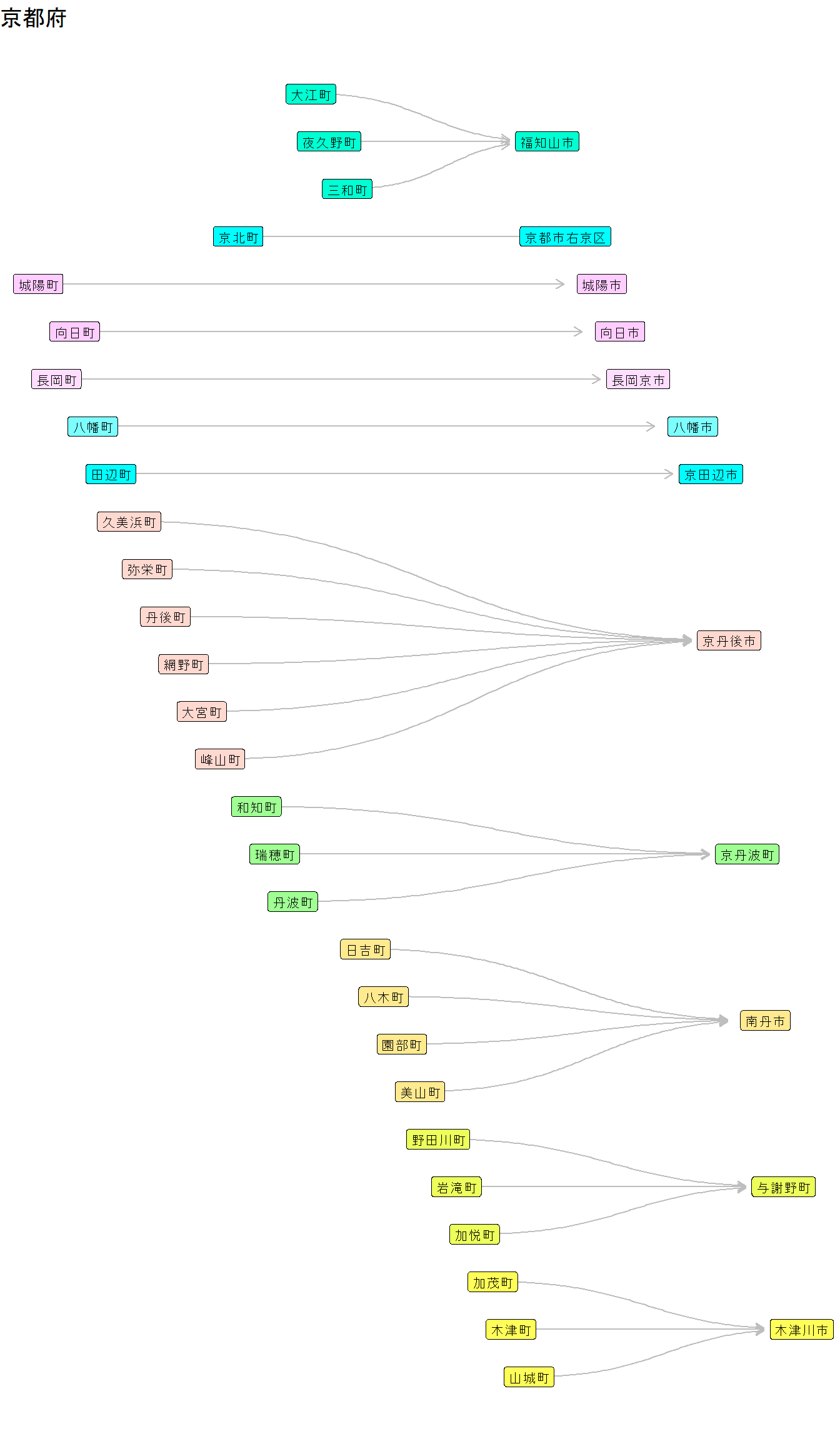
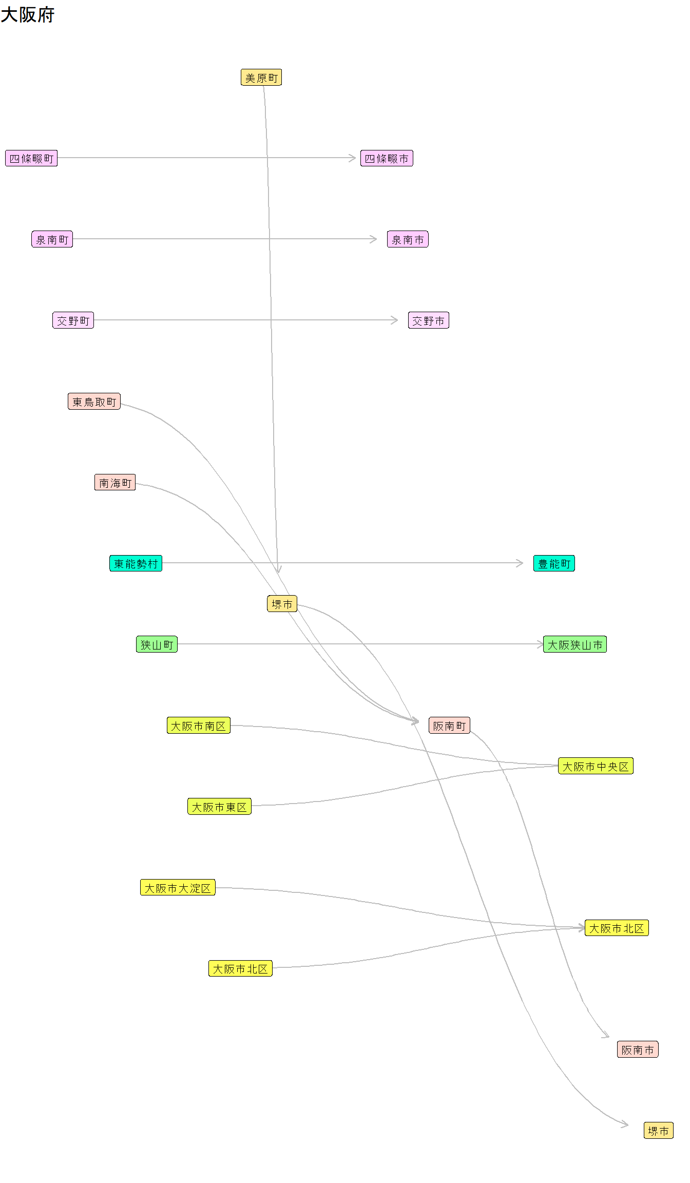
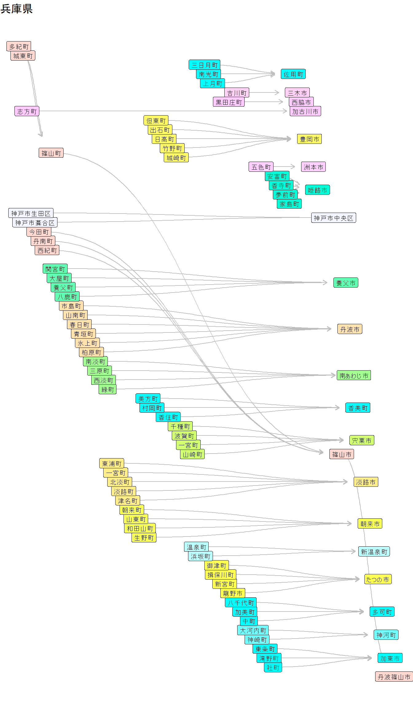
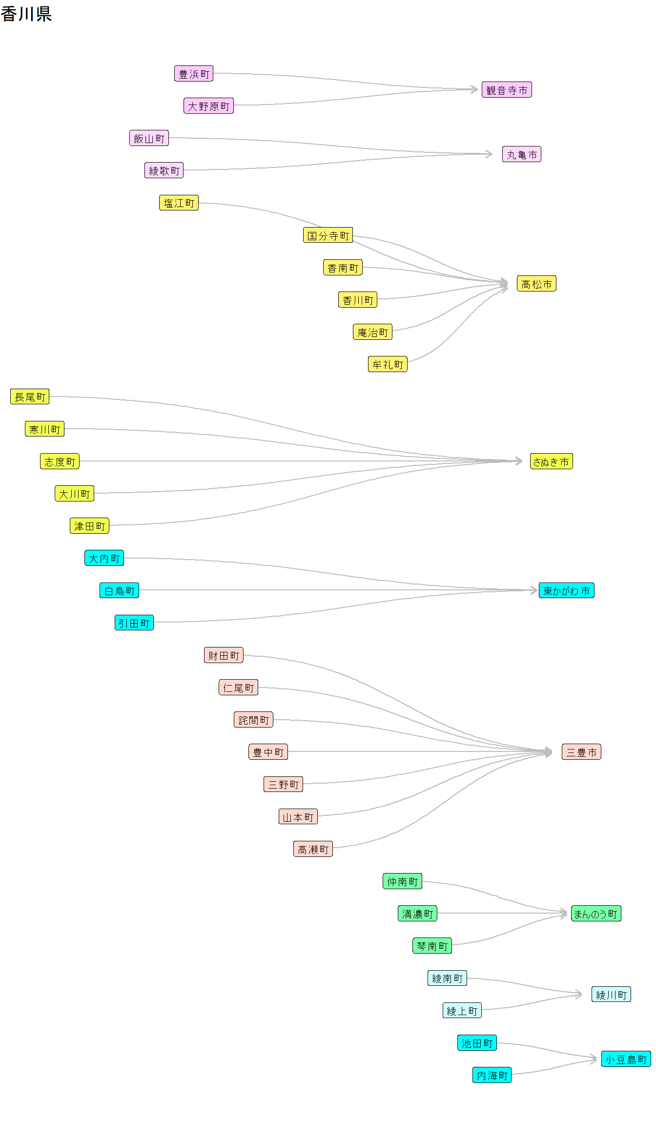
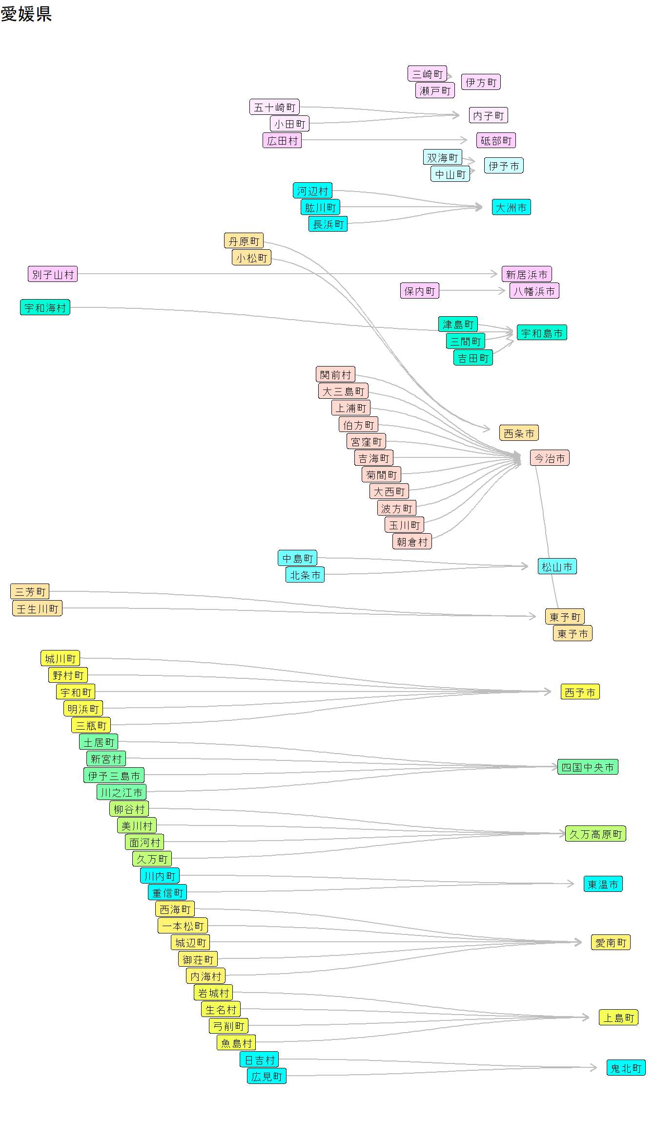
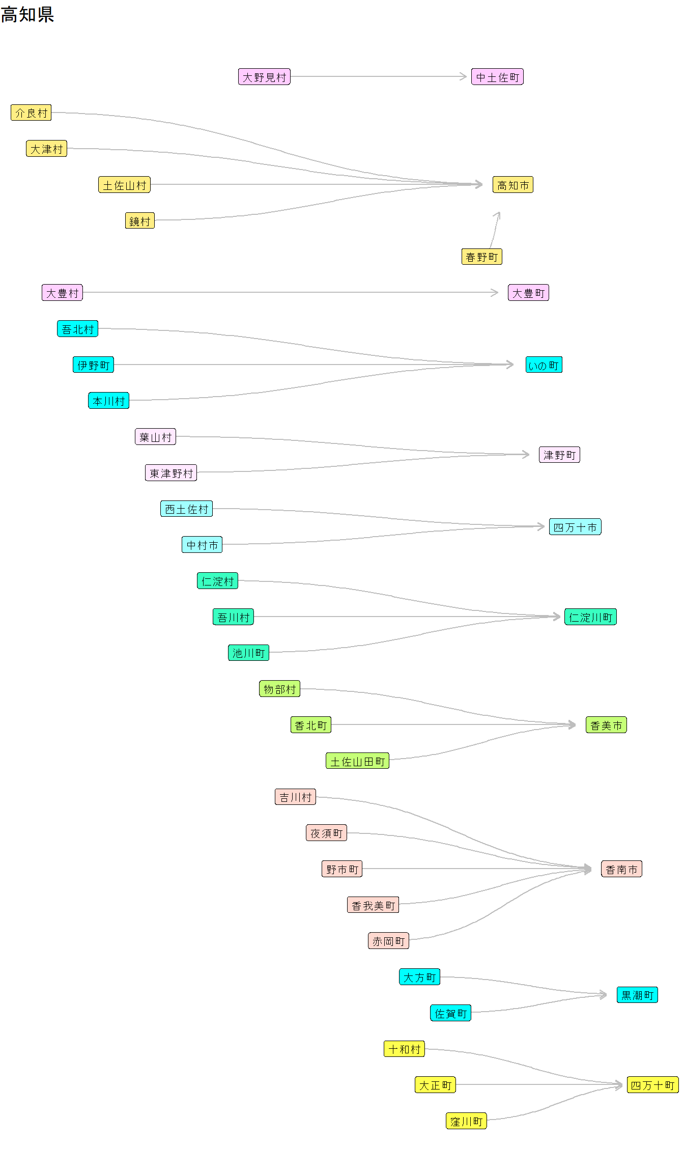
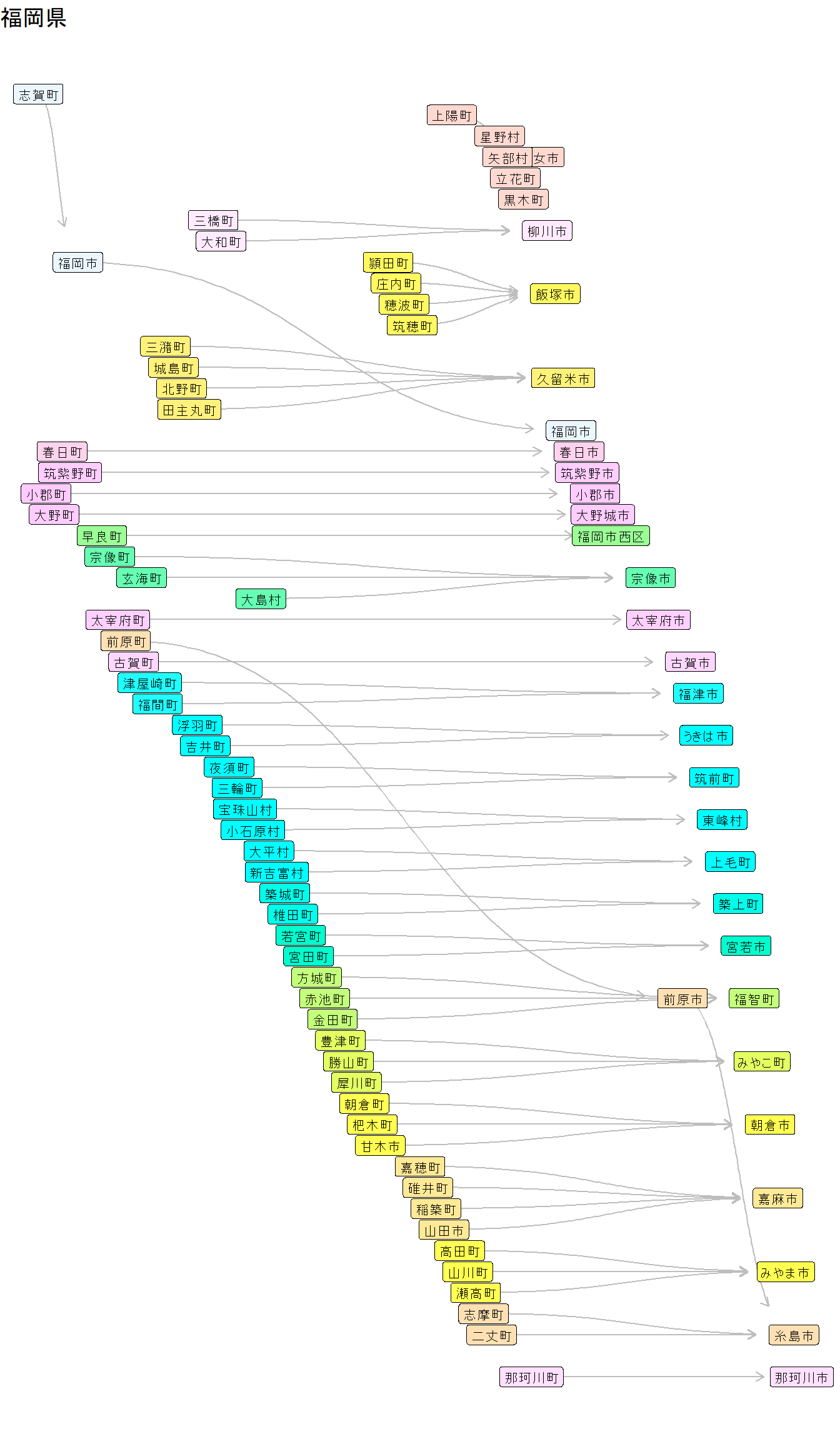
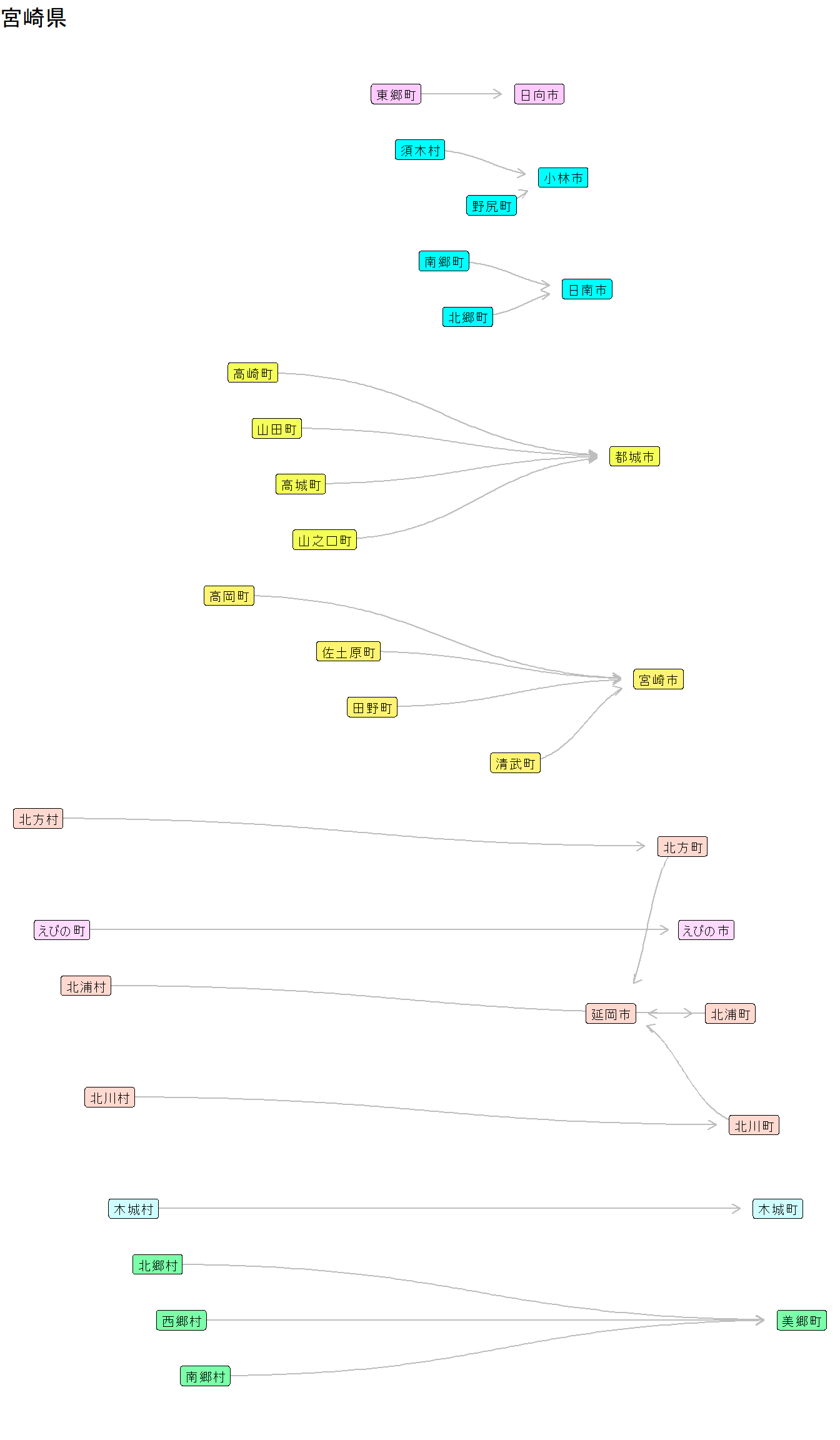
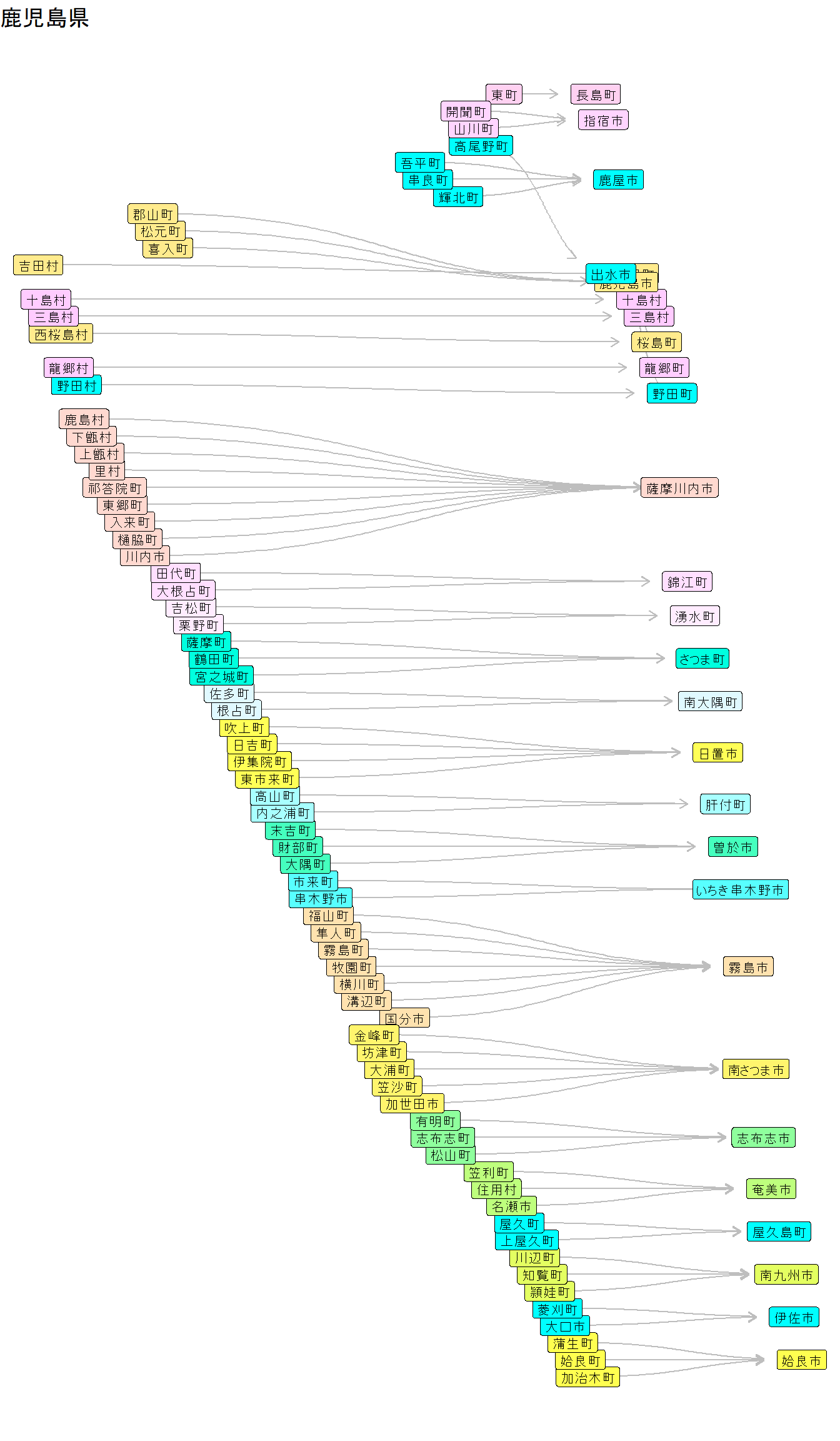
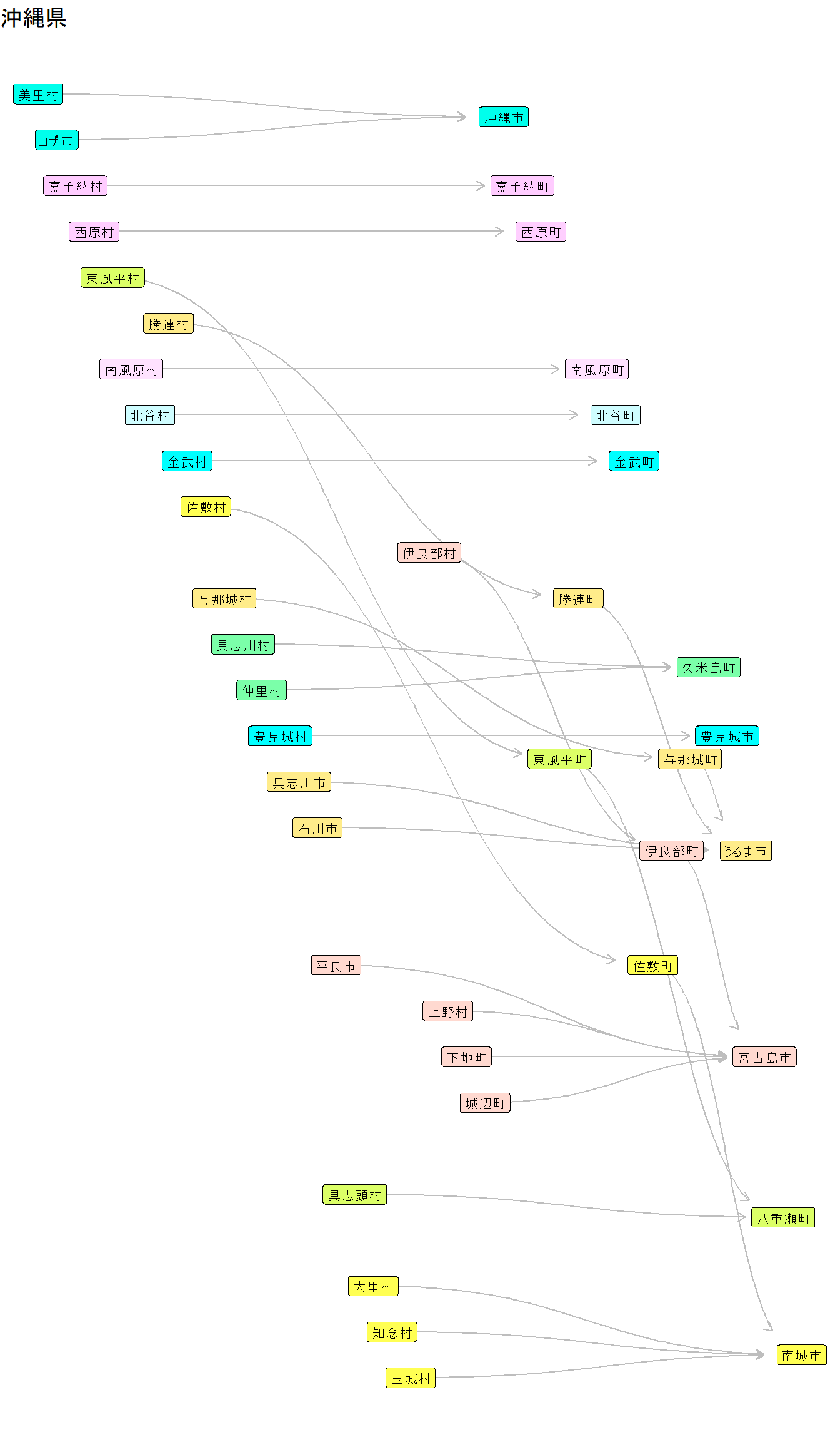
Visualization results of municipal mergers by prefecture

Below are the visualization results of municipal mergers. If you notice any issues with the data, I’d appreciate it if you could let me know in the comments. Please note that in some places the labels overlap and are hard to read.

Code

library(tidyverse)
library(tidygraph)
library(ggraph)

date_end <- ymd("2024-04-01")

graph_city <- jpcity:::graph_city$graph_city |>

  activate(nodes) |>
  filter(!node_is_isolated(),
         is.infinite(interval) | int_end(interval) <= date_end) |>
  arrange(desc(interval)) |>

  replace_na(list(city_desig_name = "",
                  city_name = "")) |>
  mutate(city_name = str_c(city_desig_name, city_name)) |>
  select(!city_desig_name) |>

  mutate(group = group_components()) |>

  activate(edges) |>
  filter(!type %in% c("分離", "分割"))

jpcity::parse_pref(1:47) |>
  walk(\(pref) {
    pref_name <- jpcity::pref_name(pref)

    plot <- graph_city |>
      activate(nodes) |>
      filter(pref_name == .env$pref_name) |>

      create_layout("fabric") |>

      # It's possible to align label positions with chronology, but this is omitted since it makes the graph harder to read
      # mutate(y = int_start(interval)) |>

      ggraph() +
      geom_edge_diagonal(color = "gray",
                         arrow = arrow(length = unit(2, 'mm')),
                         end_cap = circle(8, 'mm')) +
      geom_node_label(aes(label = city_name,
                          fill = as_factor(group)),
                      size = 3,
                      show.legend = FALSE) +
      scale_fill_hue(l = 100) +
      coord_flip() +

      labs(title = pref_name) +
      theme_void()

    print(plot)
  })