産業連関分析は,経済波及効果の算出に広く用いられている分析手法です. 日本では,国や都道府県によって,約5年に1度,産業連関表と呼ばれる統計データが 作成・公開されており,産業連関分析における基礎データとなっています.
これまで,産業連関分析では,Excel・VBAが用いられることが多かったようです.
一方で,近年は,Python・R・Juliaなどのプログラミング言語の普及が進んでいます. これらのプログラミング言語は以下のような特長を持っています.
無料で利用することができる
作業の再現性が高まりミスが修正しやすい・他者がミスに気づきやすい
高度な分析手法が簡単に利用できる
そのため今後は,産業連関分析においても,これらのプログラミング言語の利用が 進むのではないかと思われます.
ここでは,Rを用いて産業連関分析を行います. Rでは近年,tidyverseなどモダンなデータ分析を行うためのパッケージが 多く提供されており,プログラミング初心者でも習得しやすい言語であると思います.
産業連関表として,e-Statのデータベースで公開されている日本(国)の 2013年・13部門産業連関表を用います. ここで使用するデータは, こちら からダウンロードできます.
産業連関分析の基礎
産業連関分析は一般的に以下の流れに従って行われます.
産業連関表 の整形
投入係数行列 の算出
レオンチェフ逆行列 の算出
経済波及効果 の算出
まず,産業連関分析において重要な投入係数行列・レオンチェフ逆行列・経済波及効果の算出方法について解説します.
投入係数行列とは
投入係数は,産業の「クッキングレシピ 」として呼ばれており,産業\(j\) の生産物を1単位生産するのに必要な産業\(i\) の生産物の量を表すものです.具体的には,以下のように中間投入\(x_{ij}\) を生産額\(X_j\) (産出額)で割ることで算出できます.
\[
a_{ij}=\frac{x_{ij}}{X_j}
\]
産業連関分析では,「クッキングレシピ」に相当する投入係数\(a_{ij}\) に基づく生産額のバランス式(行方向)を連立方程式として解きます.そこで,以下のように,投入係数行列 (通常,\(A\) と表される)と呼ばれる行列を作成することで,連立方程式が簡単に解けるようになります.
\[
A = \begin{pmatrix}
a_{11} & \cdots & a_{1n} \\
\vdots & \ddots & \vdots \\
a_{n1} & \cdots & a_{nn} \\
\end{pmatrix}
\]
レオンチェフ逆行列による経済波及効果の推計について
生産額のバランス式(行方向)は,行列を用いて以下のように表せます.変数の意味は以下の表の通りです.
\[
AX + F + E - M = X
\]
\(A\) 投入係数行列
\(X = (X_1, \cdots, X_n) ^ \top\) 生産額ベクトル
\(F = (F_1, \cdots, F_n) ^ \top\) 最終需要ベクトル
\(E = (E_1, \cdots, E_n) ^ \top\) 移輸出ベクトル
\(M = (M_1, \cdots, M_n) ^ \top\) 移輸入ベクトル
経済波及効果の推計では,最終需要の変化が生産額に与える波及効果 を算出します.
特に,日本の産業連関表での経済波及効果の推計では,移輸入 \(M\) の扱いに注意が必要 です(これは,日本表の多くが競争移輸入型表と呼ばれる形式を採用しており,投入係数に移輸入分が含まれているためです).
最終需要による経済波及効果は,域内の生産額だけでなく域外からの移輸入を誘発すると考えられます.この効果を無視すると経済波及効果を過大評価することにつながるため,通常,投入係数から移輸入相当分を差し引く という処理が行われます.
移輸入は域内需要におおよそ比例すると考えられるため,以下のように,移輸入係数\(\hat{M_i}\) が算出できます.
\[
\hat{M_i} = \frac{M_i}{\sum_{j}a_{ij}X_j + F_i}
\]
さらに,行列での計算に適した移輸入係数行列\(\hat{M}\) が,以下のように定義されます.
\[
\hat{M} =
\begin{pmatrix}
\hat{M_1} & & 0 \\
& \ddots & \\
0 & & \hat{M_n} \\
\end{pmatrix}
\]
以上より,生産額のバランス式(行方向)は,移輸入係数行列\(\hat{M}\) を用いて,以下のように変形されます.ただし,\(I\) は単位行列(対角成分が1,それ以外が0の正方行列)です.
\[
\begin{align}
AX + F + E - \hat{M} (AX + F) &= X \\
(I - \hat{M}) (AX + F) + E &= X
\end{align}
\]
上のバランス式より,経済波及効果の算出式が,以下のように導出されます.ここで,\(\Delta X\) ,\(\Delta F\) は,それぞれ,生産額の変化量,最終需要の変化量です.
\[
\begin{align}
X &= (I - \hat{M}) (AX + F) + E \\
[I - (I - \hat{M}) A] X &= (I - \hat{M}) F + E \\
X &= [I - (I - \hat{M}) A] ^ {-1} [(I - \hat{M}) F + E] \\
\Delta X &= [I - (I - \hat{M}) A] ^ {-1} (I - \hat{M}) \Delta F
\end{align}
\]
生産額の変化量\(\Delta X\) の式の右辺の\((I - \hat{M}) \Delta F\) は,最終需要の変化量に自給率\(I - \hat{M}\) を掛けた値となっています.
また,\([I - (I - \hat{M}) A] ^ {-1}\) は,最終需要の変化による直接・間接の波及効果を表す行列であり(開放型または競争移輸入型の)レオンチェフ逆行列 と呼ばれています.
以上のように,最終需要の変化量\(\Delta F\) から生産額の変化量\(\Delta X\) を推計するというのが,最も一般的な産業連関分析の方法となっています.
Rによる産業連関分析
産業連関表の整形
ここでは, こちら からダウンロードできる日本の2011年の3部門表(iotable_3sector_2011_wider.csv)を使用します.
こちらの表は,以下のように,日本の2011年の13部門表より作成したもので,単位は「百万円」 です.
13部門の産業分類を第1次・第2次・第3次産業に集計 (注:「分類不明」を第3次産業に分類)
付加価値部門を1部門に集計
最終需要部門を域内最終需要(finaldemand)・輸出(export)・輸入(import)の3部門に集計
産業連関表のデータ形式は,e-Statのデータベースで提供されている表などを除いて, 行に投入部門(input)・列に産出部門(output)を持つ「横長データ」であることが多いと思われます.
ここでも,以下の通り,まずは横長の産業連関表データを読み込みます.
library (tidyverse)<- read_csv ("iotable_3sector_2011_wider.csv" ,col_types = cols (.default = "c" )) |> # input (投入) 列以外を数値に変換 mutate (across (! input, parse_number)):: kable (iotable_wider)
industry/01_primary
1456611
7850628
1373767
3869875
47890
-2562809
industry/02_secondary
2715710
161897553
62841827
132924323
54473273
-71673715
industry/03_tertiary
2025270
66811645
155796589
352324555
16423417
-8921553
valueadded/04_valueadded
5838371
106619145
364447740
NA
NA
NA
データ分析においては,「横長データ」よりも,以下のような「縦長データ」のほうが, 分析しやすい場合が多くあります. ここでも,横長の産業連関表を「縦長データ」に変換します.
<- iotable_wider |> # input (投入) 列を分類・名称に分割 separate (input, c ("input_type" , "input_name" ),sep = "/" ) |> # input (投入) と同様にoutput (産出) の分類・名称列を追加し縦長データに pivot_longer (! c (input_type, input_name),names_to = c ("output_type" , "output_name" ),names_sep = "/" ,values_to = "value_M" ) |> # 数値が存在しない行を削除 drop_na (value_M):: kable (iotable)
industry
01_primary
industry
01_primary
1456611
industry
01_primary
industry
02_secondary
7850628
industry
01_primary
industry
03_tertiary
1373767
industry
01_primary
finaldemand
04_finaldemand
3869875
industry
01_primary
export
05_export
47890
industry
01_primary
import
06_import
-2562809
industry
02_secondary
industry
01_primary
2715710
industry
02_secondary
industry
02_secondary
161897553
industry
02_secondary
industry
03_tertiary
62841827
industry
02_secondary
finaldemand
04_finaldemand
132924323
industry
02_secondary
export
05_export
54473273
industry
02_secondary
import
06_import
-71673715
industry
03_tertiary
industry
01_primary
2025270
industry
03_tertiary
industry
02_secondary
66811645
industry
03_tertiary
industry
03_tertiary
155796589
industry
03_tertiary
finaldemand
04_finaldemand
352324555
industry
03_tertiary
export
05_export
16423417
industry
03_tertiary
import
06_import
-8921553
valueadded
04_valueadded
industry
01_primary
5838371
valueadded
04_valueadded
industry
02_secondary
106619145
valueadded
04_valueadded
industry
03_tertiary
364447740
上で構築した表データは,各行のフィルタリングなどが容易にできる一方で, 産業連関分析に用いられる行列計算などに適していません.
そこで,表データの基本的な演算と行列計算を同時に行えるdibbleパッケージを用います. 以下のように,産業連関表をdibbleに変換します.
# pak::pak("UchidaMizuki/dibble") library (dibble)<- iotable |> dibble_by (input = c (input_type, input_name),output = c (output_type, output_name),# "_"で列名を分割してinput (投入)・output (産出) 軸を設定 .names_sep = "_" )
# A dibble:   24 x 1
# Dimensions: input [4], output [6]
# Measures:   value_M
   input$type $name        output$type $name            value_M
   <chr>      <chr>        <chr>       <chr>              <dbl>
 1 industry   01_primary   industry    01_primary       1456611
 2 industry   01_primary   industry    02_secondary     7850628
 3 industry   01_primary   industry    03_tertiary      1373767
 4 industry   01_primary   finaldemand 04_finaldemand   3869875
 5 industry   01_primary   export      05_export          47890
 6 industry   01_primary   import      06_import       -2562809
 7 industry   02_secondary industry    01_primary       2715710
 8 industry   02_secondary industry    02_secondary   161897553
 9 industry   02_secondary industry    03_tertiary     62841827
10 industry   02_secondary finaldemand 04_finaldemand 132924323
# ℹ 14 more rows
投入係数行列の算出
産業の「クッキングレシピ」と呼ばれる投入係数行列\(A\) を以下のように中間投入を生産額で割って算出します.
注:dibbleではブロードキャストが自動で行われますが,安全のため,ブロードキャストを行う際に,警告を発するように設計されています.そのため,broadcast()でブロードキャスト後の軸名c("input", "output")を与えて警告が出ないようにする必要があります.
# 生産額 <- iotable |> filter (output$ type == "industry" ) |> apply ("output" , sum)# 中間投入 <- iotable |> filter (input$ type == "industry" ,$ type == "industry" )# 投入係数 <- broadcast (interindustry / total_input,c ("input" , "output" ))
# A dibble:   9
# Dimensions: input [3], output [3]
  input$type $name        output$type $name              .
  <chr>      <chr>        <chr>       <chr>          <dbl>
1 industry   01_primary   industry    01_primary   0.121
2 industry   01_primary   industry    02_secondary 0.0229
3 industry   01_primary   industry    03_tertiary  0.00235
4 industry   02_secondary industry    01_primary   0.226
5 industry   02_secondary industry    02_secondary 0.472
6 industry   02_secondary industry    03_tertiary  0.108
7 industry   03_tertiary  industry    01_primary   0.168
8 industry   03_tertiary  industry    02_secondary 0.195
9 industry   03_tertiary  industry    03_tertiary  0.267
レオンチェフ逆行列の算出
経済波及効果を表すレオンチェフ逆行列は以下のように,移輸入係数と投入係数を用いて算出できます.
注:solve()で逆行列を算出すると行列の軸名が入れ替わるため注意してください.
# 域内需要 <- iotable |> filter (input$ type == "industry" ,! output$ type %in% c ("export" , "import" )) |> apply ("input" , sum)# (移) 輸入 <- iotable |> filter (input$ type == "industry" ,$ type == "import" ) |> apply ("input" , sum)# 符号を正に <- - import# (移) 輸入係数 <- import / localdemand<- eye (inputcoeff) # 単位行列 <- importcoeff # 移輸入係数ベクトル (broadcastが行われるため行列でなくてよい) <- inputcoeff # 投入係数行列 # レオンチェフ逆行列 <- broadcast (I - (1 - M) * A,c ("input" , "output" )) |> solve ()
# A dibble:   9
# Dimensions: output [3], input [3]
  output$type $name        input$type $name              .
  <chr>       <chr>        <chr>      <chr>          <dbl>
1 industry    01_primary   industry   01_primary   1.12
2 industry    01_primary   industry   02_secondary 0.0361
3 industry    01_primary   industry   03_tertiary  0.00716
4 industry    02_secondary industry   01_primary   0.374
5 industry    02_secondary industry   02_secondary 1.68
6 industry    02_secondary industry   03_tertiary  0.197
7 industry    03_tertiary  industry   01_primary   0.348
8 industry    03_tertiary  industry   02_secondary 0.445
9 industry    03_tertiary  industry   03_tertiary  1.41
経済波及効果の算出
こちら からダウンロードできる最終需要がそれぞれ百万円ずつ増加する(finaldemand_change_3sector.csv)ケースで経済波及効果を算出しています.
# 最終需要変化量 <- read_csv ("finaldemand_change_3sector.csv" ,col_types = cols (.default = "c" ,value_M = "n" )) |> dibble_by (input = c (input_type, input_name),.names_sep = "_" )<- leontiefinv # レオンチェフ逆行列 <- importcoeff # 移輸入係数 <- finaldemand_change # 最終需要変化量 # 経済波及効果 <- L %*% ((1 - M) * FD)
# A dibble:   3
# Dimensions: output [3]
  output$type $name            .
  <chr>       <chr>        <dbl>
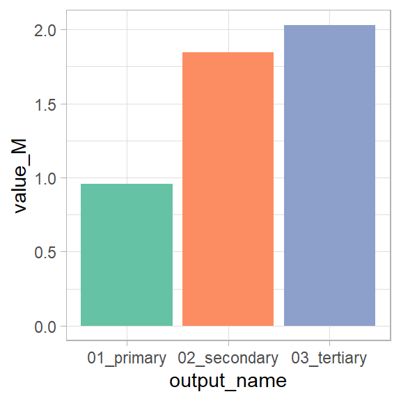
1 industry    01_primary   0.958
2 industry    02_secondary 1.85
3 industry    03_tertiary  2.03
theme_set (theme_light ())|> as_tibble (n = "value_M" ) |> unpack (output, names_sep = "_" ) |> ggplot (aes (output_name, value_M,fill = output_name)) + geom_col (show.legend = FALSE ) + scale_fill_brewer (palette = "Set2" )
まとめ
Rを用いた産業連関分析の方法について紹介しました.
ここまでの計算は,econio パッケージにまとめられています.また,econiodatajp パッケージを使うと,e-Statから産業連関表をダウンロード・整形する手間なく,そのまま産業連関表を取得できます.以下のように,ここまでの計算と同様の計算を行うことができます(なお,jpioパッケージは現在使用しておらず,econio・econiodatajpに置き換わっています).
# pak::pak("UchidaMizuki/econio") # pak::pak("UchidaMizuki/econiodatajp") library (econio)library (econiodatajp)# 産業連関表(2020年,全国,統合大分類)の取得 <- io_table_get (region_type = "regional" ,region_class = "nation" ,year = 2020 ,sector_class = "large" ,language = "ja"
# Input-output table: regional
# Dimensions:         input [43], output [47]
# Input:              43 sectors
# Output:             47 sectors
# Import type:        competitive
   input$sector           output$sector                                 .
   <sector>               <sector>                                  <dbl>
 1 <industry> 01_農林漁業 <industry> 01_農林漁業               1602100000
 2 <industry> 01_農林漁業 <industry> 06_鉱業                            0
 3 <industry> 01_農林漁業 <industry> 11_飲食料品               7253300000
 4 <industry> 01_農林漁業 <industry> 15_繊維製品                 16500000
 5 <industry> 01_農林漁業 <industry> 16_パルプ・紙・木製品      289700000
 6 <industry> 01_農林漁業 <industry> 39_その他の製造工業製品     39900000
 7 <industry> 01_農林漁業 <industry> 20_化学製品                 41700000
 8 <industry> 01_農林漁業 <industry> 21_石油・石炭製品                  0
 9 <industry> 01_農林漁業 <industry> 22_プラスチック・ゴム製品  103500000
10 <industry> 01_農林漁業 <industry> 25_窯業・土石製品             800000
# ℹ 2,011 more rows
# 投入係数 io_input_coef (iotable)
Assuming `open_economy = FALSE`.
# Input-output table: regional
# Dimensions:         input [37], output [37]
# Input:              37 sectors
# Output:             37 sectors
# Import type:        competitive
   input$sector           output$sector                               .
   <sector>               <sector>                                <dbl>
 1 <industry> 01_農林漁業 <industry> 01_農林漁業               0.130
 2 <industry> 01_農林漁業 <industry> 06_鉱業                   0
 3 <industry> 01_農林漁業 <industry> 11_飲食料品               0.191
 4 <industry> 01_農林漁業 <industry> 15_繊維製品               0.00568
 5 <industry> 01_農林漁業 <industry> 16_パルプ・紙・木製品     0.0253
 6 <industry> 01_農林漁業 <industry> 39_その他の製造工業製品   0.00455
 7 <industry> 01_農林漁業 <industry> 20_化学製品               0.00147
 8 <industry> 01_農林漁業 <industry> 21_石油・石炭製品         0
 9 <industry> 01_農林漁業 <industry> 22_プラスチック・ゴム製品 0.00756
10 <industry> 01_農林漁業 <industry> 25_窯業・土石製品         0.000122
# ℹ 1,359 more rows
# レオンチェフ逆行列 io_leontief_inverse (iotable)
Assuming `open_economy = FALSE`.
# Input-output table: regional
# Dimensions:         output [37], input [37]
# Input:              37 sectors
# Output:             37 sectors
# Import type:        competitive
   output$sector          input$sector                                .
   <sector>               <sector>                                <dbl>
 1 <industry> 01_農林漁業 <industry> 01_農林漁業               1.19
 2 <industry> 01_農林漁業 <industry> 06_鉱業                   0.000704
 3 <industry> 01_農林漁業 <industry> 11_飲食料品               0.286
 4 <industry> 01_農林漁業 <industry> 15_繊維製品               0.0116
 5 <industry> 01_農林漁業 <industry> 16_パルプ・紙・木製品     0.0436
 6 <industry> 01_農林漁業 <industry> 39_その他の製造工業製品   0.0108
 7 <industry> 01_農林漁業 <industry> 20_化学製品               0.00860
 8 <industry> 01_農林漁業 <industry> 21_石油・石炭製品         0.000467
 9 <industry> 01_農林漁業 <industry> 22_プラスチック・ゴム製品 0.0136
10 <industry> 01_農林漁業 <industry> 25_窯業・土石製品         0.00202
# ℹ 1,359 more rows
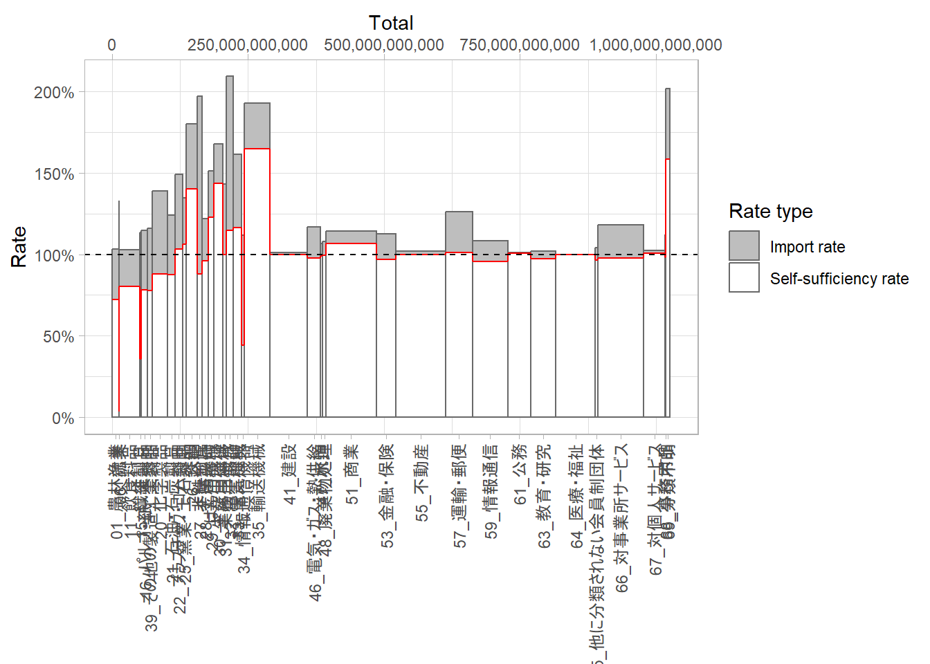
# スカイラインチャート autoplot (iotable, type = "skyline" )
特定の最終需要変化に対する経済波及効果は,econioには専用の関数は用意されていないため,上記で紹介したように,レオンチェフ逆行列に最終需要の変化量を掛け合わせることで算出します.