library(tidyverse)
library(dm)
library(repurrrsive)Note: This article is a machine-translated translation of my Japanese article with simple modifications.
How do we reduce errors in data preprocessing?
It is said that 80% of the time required for data analysis is spent on preprocessing. Even though preprocessing determines the quality of subsequent data analysis, the more time spent on pre-processing means the probability of making mistakes is also high.
Preprocessing tasks include “extraction,” “aggregation,” and “joining (merging)” of data frames. Among these, data joining is a task that tends to make the code longer and more prone to errors. And since the data frames needed for analysis are rarely combined into one, joining data frames is a widespread process.
Typical mistakes that tend to occur when joining data frames are as follows1,
- The keys of the data frame to be joined are not “MECE”
- Mistaken keys to join data frames
If you have experienced any mistakes or near-misses in joining data frames, you may be better off relying on some sort of package instead of letting them go unattended. Besides, even if there were no mistakes, we tend to be skeptical about whether we did the right thing in the past.
This article introduces the R dm package, a powerful solution to the problems of errors and skepticism in joining data frames.
Relational data model with dm
The relational data model provided by dm manages the relationships among multiple data on our behalf.
This article describes the use and advantages of the relational data model provided by dm. the Star Wars data set provided by the repurrrsive package. For this purpose, let’s use the Star Wars dataset provided by the repurrrsive package. tidyverse, dm, and repurrrsive packages must be pre-loaded.
The Star Wars dataset provided by repurrrsive includes the followings2.
StarWars dataset provided by repurrrsive
data(package = "repurrrsive") |>
  chuck("results") |>
  as_tibble() |>
  filter(str_starts(Item, "sw_")) |>
  pull(Item)
[1] "sw_films" "sw_people" "sw_planets" "sw_species" "sw_starships"
[6] "sw_vehicles" This article will illustrate the use of the relational data model through the following two analytical examples. These examples require dealing with relationships among multiple data sets.
- Basic: Building a relational data model with dm
- Application: Extending the model and validating keys with dm
1. Basic: Building a relational data model with dm
As a basic example, let us build a relational data model to determine the composition ratio of the home planets of the characters in Star Wars movies. To perform this analysis, three data frames, films, people, and planets, are prepared as shown below. Here, only the necessary data are selected to simplify the analysis3.
films <- tibble(film = sw_films) |>
  unnest_wider(film) |>
  select(url, title, characters)
people <- tibble(person = sw_people) |>
  unnest_wider(person) |>
  select(url, name, homeworld, species)
planets <- tibble(planet = sw_planets) |>
  unnest_wider(planet) |>
select(url, name)filmspeopleplanetsChecking the prepared data frames, we can see that url column of each data frame is used as a key, so the relationship between the data frames can be summarized as shown in the following figure4.
Since it is common for a film to have multiple characters, it is important to note that characters column of films is a list of characters, so it isn’t possible to join characters column of films to url column of people.
flowchart TB
  films.characters --> people.url
  people.homeworld --> planets.url
  subgraph films
    films.url[url]
    films.title[title]
    films.characters[List of characters]
  end
  subgraph people
    people.url[url]
    people.name[name]
    people.homeworld[homeworld]
  end
  subgraph planets
    planets.url[url]
    planets.name[name]
  end
Therefore, we consider creating a new data file, films_x_characters, that represents the relationship between films and people, i.e., which characters appear in which films5.Through films_x_characters, the relationship between data can be summarized as shown in the following figure.
flowchart TB
  films_x_characters.url --> films.url
  films_x_characters.characters ---> people.url
  people.homeworld --> planets.url
  subgraph films_x_characters
    films_x_characters.url[url]
    films_x_characters.characters[characters]
  end
  subgraph films
    films.url[url]
    films.title[title]
  end
  subgraph people
    people.url[url]
    people.name[name]
    people.homeworld[homeworld]
  end
  subgraph planets
    planets.url[url]
    planets.name[name]
  end
Now, let’s build a relational data model according to the above image. First, create films_x_characters using url and characters columns of films. In addition, I delete the unnecessary characters column from films.
# Create films_x_characters and remove characters column from films
films_x_characters <- films |>
  select(url, characters) |>
  unnest_longer(characters)
films <- films |>
  select(!characters)

films_x_characters
Finally, after passing the prepared films, people, planets, and films_x_characters to dm(), a relational data model can be built by adding primary keys and foreign keys.
In dm, primary keys are set with dm_add_pk()6 and foreign keys with dm_add_fk()7.
dm_starwars_1 <- dm(films, people, planets, films_x_characters) |>

  # 1. Add primary keys
  dm_add_pk(films, url) |>
  dm_add_pk(people, url) |>
  dm_add_pk(planets, url) |>
  dm_add_pk(films_x_characters, c(url, characters)) |>

  # 2. Add foreign keys
  dm_add_fk(films_x_characters, url, films) |>
  dm_add_fk(films_x_characters, characters, people) |>
  dm_add_fk(people, homeworld, planets)

dm_starwars_1
── Metadata ────────────────────────────────────────────────────────────────────
Tables: `films`, `people`, `planets`, `films_x_characters`
Columns: 10
Primary keys: 4
Foreign keys: 3The relational data model can be drawn using dm_draw(). The drawing reveals that the same relationships are built as in the image above.
dm_draw(dm_starwars_1)By using dm_flatten_to_tbl() as shown below, a data frame can be created by joining films_x_characters data with films/people/planets data. In this case, if the same column names exist between different data, the column names are automatically renamed according to the data names. In this way, the relational data model manages the relationships between data on our behalf, allowing us to automatically join data frames based on the relationships among other data.
data_films_x_characters_1 <- dm_starwars_1 |>
  dm_flatten_to_tbl(films_x_characters,
                    .recursive = TRUE)
Renaming ambiguous columns: %>%
dm_rename(people, name.people = name) %>%
dm_rename(planets, name.planets = name)data_films_x_characters_1The data_films_x_characters_1 can be used to plot the composition ratio of the characters’ home planets, as shown below. We will not discuss this plot further. However, we have confirmed that the relational data model can be used to automate the joining of data frames.
In the above analysis, it is easy to join data frames using left_join(), and you may not see the advantage of using a relational data model. In the application section, we will consider a more complex situation where a relational data model prevails.
Plot of the composition of the characters’ home planets
data_films_x_characters_1 |>
  mutate(name.planets = fct_lump_n(name.planets, 7,
                                   ties.method = "first") |>
           fct_relevel("Other",
                       after = Inf)) |>
  count(title, name.planets) |>
  mutate(prop = n / sum(n),
         .by = title,
         .keep = "unused") |>
  ggplot(aes(fct_rev(title), prop,
             fill = name.planets)) +
  geom_col(position = position_stack(reverse = TRUE)) +
  geom_text(aes(label = if_else(prop < 5e-2,
                                "",
                                scales::label_percent(accuracy = 1)(prop))),
            position = position_stack(vjust = 0.5,
                                      reverse = TRUE)) +
  scale_x_discrete("Title") +
  scale_y_continuous("Composition of the characters' home planets",
                     labels = scales::percent) +
  scale_fill_brewer("Planet Name",
                    palette = "Set2") +
  coord_flip() +
  theme(legend.position = "bottom") +
  guides(fill = guide_legend(nrow = 2,
                             byrow = TRUE))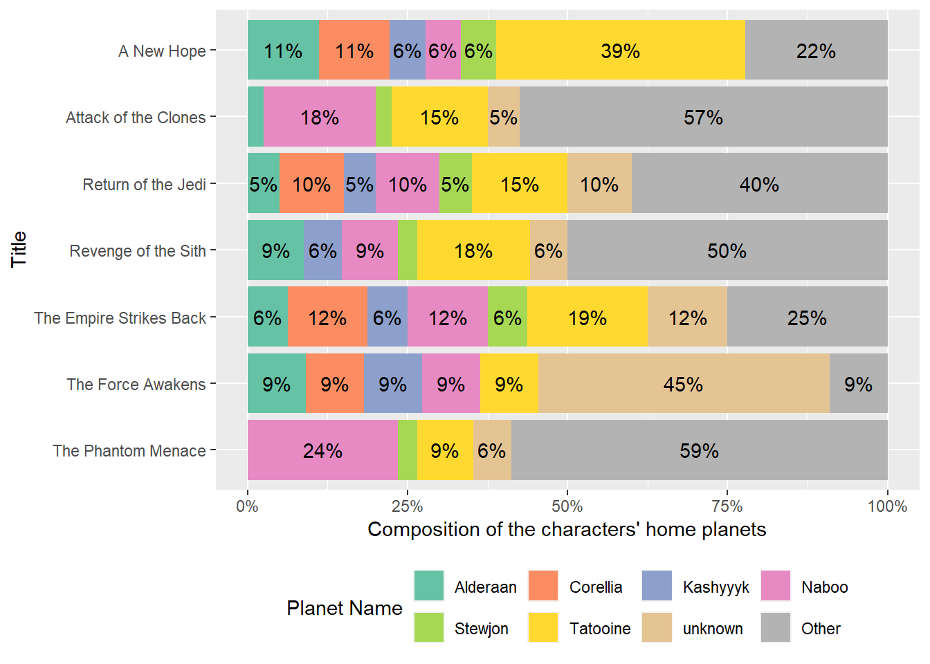
2. Application: Extending the model and validating keys with dm
In the application, we will examine the composition ratio of the species of the characters in Star Wars movies. The difficulty level of this analysis is not much different from that of the basic analysis. However, as the amount of data to be handled increases, the code tends to become more complicated, and the advantages of using a relational data model are significant. In addition, the advantages of the relational data model include the following,
- New data can be added to the existing relational data model
- Possible to check key constraints defined to join data frames
We prepare in advance the species data needed for this analysis.
species <- tibble(species = sw_species) |>
  unnest_wider(species) |>
  select(url, name)

species
In dm, we can add new data to the relational data model using dm(). In this example, let’s build dm_starwars_2 by adding the species data to dm_starwars_1. By using dm_draw(), we can see that the model has been updated.
dm_starwars_2 <- dm_starwars_1 |>
  dm(species) |>
  dm_add_pk(species, url) |>
  dm_add_fk(people, species, species)

dm_draw(dm_starwars_2)
Next, let us check key constraints to join data frames. This can be done using dm_examine_constraints(). Let’s check the behavior of dm_examine_constraints() by building a model that contains the two types of mistakes mentioned above as common mistakes. Here, dm_starwars_2_strong_data is data in which the first row of the species data has been deleted and the data is not “MECE”. dm_starwars_2_wrong_pk is the data with the wrong primary key in the species data.
dm_starwars_2_wrong_data <- dm_starwars_1 |>
  dm(species = species |>
       slice(-1)) |>
  dm_add_pk(species, url) |>
  dm_add_fk(people, species, species)

dm_starwars_2_wrong_pk <- dm_starwars_1 |>
  dm(species) |>
  dm_add_pk(species, name) |>
  dm_add_fk(people, species, species)
Let’s look at the result of dm_examine_constraints(). For the correct model, dm_starwars_2, the message ℹ All constraints satisfied. is displayed. On the other hand, dm_starwars_2_strong_data and dm_starwars_2_strong_pk show the message ! Unsatisfied constraints: is displayed. This is because the primary key of the species data does not contain data that should be included. Thus, we see that dm_examine_constraints() can be used to easily check the key constraints.
print(dm_examine_constraints(dm_starwars_2))ℹ All constraints satisfied.print(dm_examine_constraints(dm_starwars_2_wrong_data))! Unsatisfied constraints:• Table `people`: foreign key `species` into table `species`: values of `people$species` not in `species$url`: http://swapi.co/api/species/5/ (1)print(dm_examine_constraints(dm_starwars_2_wrong_pk))! Unsatisfied constraints:• Table `people`: foreign key `species` into table `species`: values of `people$species` not in `species$name`: http://swapi.co/api/species/1/ (35), http://swapi.co/api/species/2/ (5), http://swapi.co/api/species/12/ (3), http://swapi.co/api/species/15/ (2), http://swapi.co/api/species/22/ (2), …As described above, we have seen that we can add new data to the relational data model with dm() and check key constraints with dm_examine_constraints(). Finally, the following figure shows a composition of the species of the characters in the Star Wars films using dm_starwars_2. Again, we omit the discussion of the plots.
Plot of the composition of the characters’ races
dm_starwars_2 |>
  dm_flatten_to_tbl(films_x_characters,
                    .recursive = TRUE) |>
  mutate(name.species = name.species |>
           fct_na_value_to_level("Other") |>
           fct_lump_n(7,
                      ties.method = "first") |>
           fct_relevel("Other",
                       after = Inf)) |>
  count(title, name.species) |>
  mutate(prop = n / sum(n),
         .by = title,
         .keep = "unused") |>
  ggplot(aes(fct_rev(title), prop,
             fill = name.species)) +
  geom_col(position = position_stack(reverse = TRUE)) +
  geom_text(aes(label = if_else(prop < 5e-2,
                                "",
                                scales::label_percent(accuracy = 1)(prop))),
            position = position_stack(vjust = 0.5,
                                      reverse = TRUE)) +
  scale_x_discrete("Title") +
  scale_y_continuous("Composition of the characters' races",
                     labels = scales::percent) +
  scale_fill_brewer("Species name",
                    palette = "Set2") +
  coord_flip() +
  theme(legend.position = "bottom") +
  guides(fill = guide_legend(nrow = 2,
                             byrow = TRUE))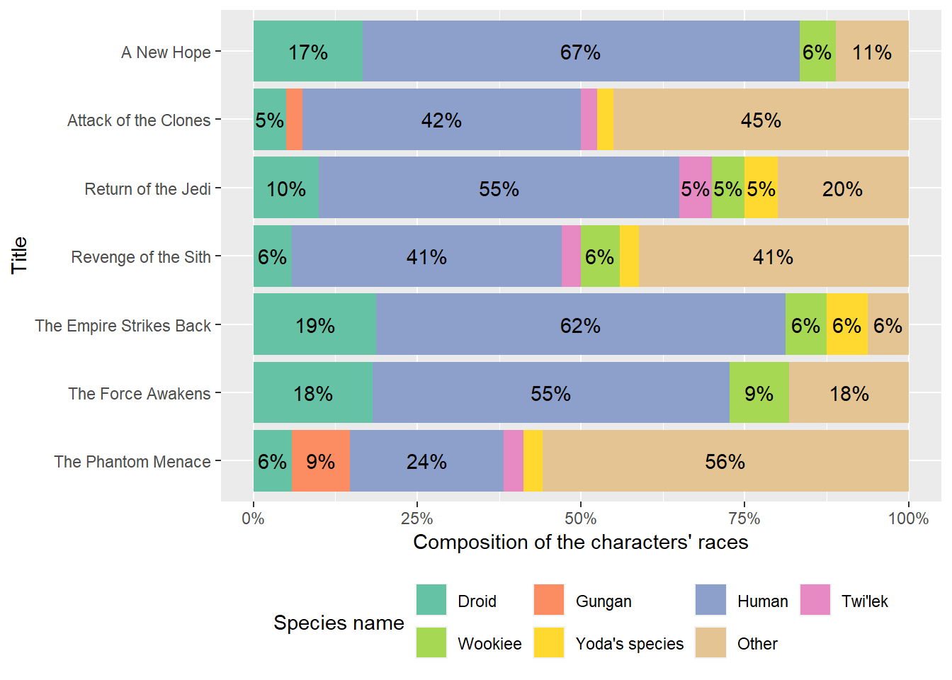
Summary
In this article, we have shown how to build a relational data model using dm. Once a relational data model is built using dm, it is no longer necessary to manage relationships among data by oneself, and data can be automatically joined using dm_flatten_to_tbl(). In addition, dm provides other useful functions to enhance the quality of data preprocessing, such as adding data to the model with dm() and checking key constraints with dm_examine_constraints().
References
- dm package site
- Preprocessing Compendium [Practical SQL/R/Python techniques for data analysis] (in Japanese)
- starwarsdb
- Star Wars relational data model available for download from CRAN
Footnotes
Fortunately, recent versions of dplyr warn against duplicate keys when joining data frames.↩︎
Among the data exported by repurrrsive, the data whose name begins with
sw_are related to StarWars, and the part aftersw_represents the content of the data.↩︎The
speciescolumn ofsw_peopleis not needed here, but is selected for use in the next analysis.↩︎Here, I used mermaid to illustrate the relationship between data frames.↩︎
There is no clear hierarchical relationship between works and characters, so the name
characters_x_filmsis acceptable.↩︎For
films,people, andplanets, theurlcolumn is the primary key, and forfilms_x_characters,urlandcharactersare the primary keys.↩︎Following the arrows in the image above, I set foreign keys.↩︎