Input-output analysis is a widely used analytical method for calculating economic ripple effects. In Japan, statistical data called input-output tables are compiled and published roughly once every five years by the national government and prefectures, and these tables serve as the basic data for input-output analysis.
Until now, Excel and VBA have often been used for input-output analysis.
On the other hand, in recent years, programming languages such as Python, R, and Julia have become increasingly widespread. These programming languages have the following characteristics.
They can be used free of charge
Reproducibility of work is improved, making mistakes easier to fix and easier for others to notice
Advanced analytical methods can be used easily
For these reasons, it seems likely that the use of these programming languages will spread further in input-output analysis going forward.
Here, we will perform input-output analysis using R. In recent years, R has come to offer many packages, such as tidyverse, for modern data analysis, and I think it is a language that is easy to learn even for programming beginners.
As the input-output table, we use Japan’s (national) 2013 13-sector input-output table, published in the e-Stat database. The data used here can be downloaded from here.
Basics of input-output analysis
Input-output analysis is generally carried out according to the following flow.
Formatting the input-output table
Calculating the input coefficient matrix
Calculating the Leontief inverse matrix
Calculating the economic ripple effect
First, let’s explain the calculation methods for the input coefficient matrix, the Leontief inverse matrix, and the economic ripple effect, which are important in input-output analysis.
What is the input coefficient matrix?
The input coefficient is often referred to as the industry’s “cooking recipe,” and it represents the amount of output of industry \(i\) required to produce one unit of output of industry \(j\). Specifically, it can be calculated by dividing intermediate input \(x_{ij}\) by output \(X_j\) (production value), as shown below.
\[
a_{ij}=\frac{x_{ij}}{X_j}
\]
In input-output analysis, a system of simultaneous equations representing the balance of production values (in the row direction), based on the input coefficient \(a_{ij}\) corresponding to the “cooking recipe,” is solved. To make this system of simultaneous equations easy to solve, a matrix called the input coefficient matrix (usually denoted \(A\)) is constructed as follows.
Estimating economic ripple effects using the Leontief inverse matrix
The balance equation for production values (in the row direction) can be expressed using matrices as follows. The meanings of the variables are as shown in the table below.
\[
AX + F + E - M = X
\]
Variable
Meaning
\(A\)
Input coefficient matrix
\(X = (X_1, \cdots, X_n) ^ \top\)
Production value vector
\(F = (F_1, \cdots, F_n) ^ \top\)
Final demand vector
\(E = (E_1, \cdots, E_n) ^ \top\)
Interregional exports vector
\(M = (M_1, \cdots, M_n) ^ \top\)
Interregional imports vector
In estimating economic ripple effects, we calculate the ripple effect that a change in final demand has on production value.
In particular, when estimating economic ripple effects using Japanese input-output tables, care must be taken in how interregional imports\(M\)are handled (this is because most Japanese tables adopt a format called the competitive-import type, in which the interregional import portion is included in the input coefficients).
Economic ripple effects caused by final demand are thought to induce interregional imports from outside the region, in addition to production within the region. Ignoring this effect would lead to an overestimation of the economic ripple effect, so it is standard practice to subtract the portion corresponding to interregional imports from the input coefficients.
Since interregional imports are thought to be roughly proportional to demand within the region, the interregional import coefficient \(\hat{M_i}\) can be calculated as follows.
From the above, the balance equation for production values (in the row direction) can be transformed using the interregional import coefficient matrix \(\hat{M}\) as follows, where \(I\) is the identity matrix (a square matrix with 1s on the diagonal and 0s elsewhere).
\[
\begin{align}
AX + F + E - \hat{M} (AX + F) &= X \\
(I - \hat{M}) (AX + F) + E &= X
\end{align}
\]
From the balance equation above, the formula for calculating the economic ripple effect is derived as follows, where \(\Delta X\) and \(\Delta F\) are the amount of change in production value and the amount of change in final demand, respectively.
\[
\begin{align}
X &= (I - \hat{M}) (AX + F) + E \\
[I - (I - \hat{M}) A] X &= (I - \hat{M}) F + E \\
X &= [I - (I - \hat{M}) A] ^ {-1} [(I - \hat{M}) F + E] \\
\Delta X &= [I - (I - \hat{M}) A] ^ {-1} (I - \hat{M}) \Delta F
\end{align}
\]
On the right-hand side of the equation for the change in production value \(\Delta X\), \((I - \hat{M}) \Delta F\) is the value obtained by multiplying the change in final demand by the self-sufficiency rate \(I - \hat{M}\).
Also, \([I - (I - \hat{M}) A] ^ {-1}\) is a matrix representing the direct and indirect ripple effects resulting from a change in final demand, and it is called the (open, or competitive-import type) Leontief inverse matrix.
As described above, estimating the change in production value \(\Delta X\) from the change in final demand \(\Delta F\) is the most common method of input-output analysis.
Input-output analysis in R
Formatting the input-output table
Here, we use the 2011 3-sector table for Japan (iotable_3sector_2011_wider.csv), which can be downloaded from here.
This table is created from Japan’s 2011 13-sector table as follows, and the unit is “million yen”.
The 13 industry sectors are aggregated into primary, secondary, and tertiary industries (Note: “unclassifiable” is categorized as tertiary industry)
The value-added sectors are aggregated into a single sector
The final demand sectors are aggregated into three sectors: final demand within the region (finaldemand), exports (export), and imports (import)
Except for tables such as those provided in the e-Stat database, input-output table data is often provided in a “wide” format, with input sectors (input) in the rows and output sectors (output) in the columns.
Here too, we first load the wide-format input-output table data as follows.
library(tidyverse)iotable_wider <-read_csv("iotable_3sector_2011_wider.csv",col_types =cols(.default ="c")) |># Convert columns other than input to numericmutate(across(!input, parse_number))knitr::kable(iotable_wider)
input
industry/01_primary
industry/02_secondary
industry/03_tertiary
finaldemand/04_finaldemand
export/05_export
import/06_import
industry/01_primary
1456611
7850628
1373767
3869875
47890
-2562809
industry/02_secondary
2715710
161897553
62841827
132924323
54473273
-71673715
industry/03_tertiary
2025270
66811645
155796589
352324555
16423417
-8921553
valueadded/04_valueadded
5838371
106619145
364447740
NA
NA
NA
In data analysis, “long” data as shown below is often easier to work with than “wide” data. Here too, we convert the wide-format input-output table into “long” data.
iotable <- iotable_wider |># Split the input column into type and nameseparate(input, c("input_type", "input_name"),sep ="/") |># Add type/name columns for output, as with input, to create long-format datapivot_longer(!c(input_type, input_name),names_to =c("output_type", "output_name"),names_sep ="/",values_to ="value_M") |># Remove rows with no numeric valuedrop_na(value_M)knitr::kable(iotable)
input_type
input_name
output_type
output_name
value_M
industry
01_primary
industry
01_primary
1456611
industry
01_primary
industry
02_secondary
7850628
industry
01_primary
industry
03_tertiary
1373767
industry
01_primary
finaldemand
04_finaldemand
3869875
industry
01_primary
export
05_export
47890
industry
01_primary
import
06_import
-2562809
industry
02_secondary
industry
01_primary
2715710
industry
02_secondary
industry
02_secondary
161897553
industry
02_secondary
industry
03_tertiary
62841827
industry
02_secondary
finaldemand
04_finaldemand
132924323
industry
02_secondary
export
05_export
54473273
industry
02_secondary
import
06_import
-71673715
industry
03_tertiary
industry
01_primary
2025270
industry
03_tertiary
industry
02_secondary
66811645
industry
03_tertiary
industry
03_tertiary
155796589
industry
03_tertiary
finaldemand
04_finaldemand
352324555
industry
03_tertiary
export
05_export
16423417
industry
03_tertiary
import
06_import
-8921553
valueadded
04_valueadded
industry
01_primary
5838371
valueadded
04_valueadded
industry
02_secondary
106619145
valueadded
04_valueadded
industry
03_tertiary
364447740
The table data constructed above makes it easy to filter each row, but it is not well suited to the matrix computations used in input-output analysis.
Therefore, we use the dibble package, which allows us to perform both basic table operations and matrix computations at the same time. As shown below, we convert the input-output table into a dibble.
# pak::pak("UchidaMizuki/dibble")library(dibble)iotable <- iotable |>dibble_by(input =c(input_type, input_name),output =c(output_type, output_name),# Split column names on "_" to set the input/output axes.names_sep ="_")iotable
# A dibble:   24 x 1
# Dimensions: input [4], output [6]
# Measures:   value_M
   input$type $name        output$type $name            value_M
   <chr>      <chr>        <chr>       <chr>              <dbl>
 1 industry   01_primary   industry    01_primary       1456611
 2 industry   01_primary   industry    02_secondary     7850628
 3 industry   01_primary   industry    03_tertiary      1373767
 4 industry   01_primary   finaldemand 04_finaldemand   3869875
 5 industry   01_primary   export      05_export          47890
 6 industry   01_primary   import      06_import       -2562809
 7 industry   02_secondary industry    01_primary       2715710
 8 industry   02_secondary industry    02_secondary   161897553
 9 industry   02_secondary industry    03_tertiary     62841827
10 industry   02_secondary finaldemand 04_finaldemand 132924323
# ℹ 14 more rows
Calculating the input coefficient matrix
We calculate the input coefficient matrix \(A\), known as the industry’s “cooking recipe,” by dividing intermediate input by production value, as follows.
Note: In dibble, broadcasting is performed automatically, but for safety it is designed to issue a warning whenever broadcasting occurs. Therefore, you need to pass the axis names after broadcasting, c("input", "output"), to broadcast() to prevent the warning from being issued.
# A dibble:   9
# Dimensions: input [3], output [3]
  input$type $name        output$type $name              .
  <chr>      <chr>        <chr>       <chr>          <dbl>
1 industry   01_primary   industry    01_primary   0.121
2 industry   01_primary   industry    02_secondary 0.0229
3 industry   01_primary   industry    03_tertiary  0.00235
4 industry   02_secondary industry    01_primary   0.226
5 industry   02_secondary industry    02_secondary 0.472
6 industry   02_secondary industry    03_tertiary  0.108
7 industry   03_tertiary  industry    01_primary   0.168
8 industry   03_tertiary  industry    02_secondary 0.195
9 industry   03_tertiary  industry    03_tertiary  0.267
Calculating the Leontief inverse matrix
The Leontief inverse matrix, which represents the economic ripple effect, can be calculated using the interregional import coefficient and the input coefficient, as follows.
Note: Be careful, since calculating the inverse matrix with solve() swaps the axis names of the matrix.
# Demand within the regionlocaldemand <- iotable |>filter(input$type =="industry",!output$type %in%c("export", "import")) |>apply("input", sum)# (Interregional) importsimport <- iotable |>filter(input$type =="industry", output$type =="import") |>apply("input", sum)# Make the sign positiveimport <--import# (Interregional) import coefficientimportcoeff <- import / localdemandI <-eye(inputcoeff) # Identity matrixM <- importcoeff # Interregional import coefficient vector (does not need to be a matrix, since broadcasting is performed)A <- inputcoeff # Input coefficient matrix# Leontief inverse matrixleontiefinv <-broadcast(I - (1- M) * A,c("input", "output")) |>solve()leontiefinv
# A dibble:   9
# Dimensions: output [3], input [3]
  output$type $name        input$type $name              .
  <chr>       <chr>        <chr>      <chr>          <dbl>
1 industry    01_primary   industry   01_primary   1.12
2 industry    01_primary   industry   02_secondary 0.0361
3 industry    01_primary   industry   03_tertiary  0.00716
4 industry    02_secondary industry   01_primary   0.374
5 industry    02_secondary industry   02_secondary 1.68
6 industry    02_secondary industry   03_tertiary  0.197
7 industry    03_tertiary  industry   01_primary   0.348
8 industry    03_tertiary  industry   02_secondary 0.445
9 industry    03_tertiary  industry   03_tertiary  1.41
Calculating the economic ripple effect
We calculate the economic ripple effect for the case (finaldemand_change_3sector.csv, which can be downloaded from here) in which final demand increases by one million yen in each sector.
# Amount of change in final demandfinaldemand_change <-read_csv("finaldemand_change_3sector.csv",col_types =cols(.default ="c",value_M ="n")) |>dibble_by(input =c(input_type, input_name),.names_sep ="_")L <- leontiefinv # Leontief inverse matrixM <- importcoeff # Interregional import coefficientFD <- finaldemand_change # Amount of change in final demand# Economic ripple effectspillover <- L %*% ((1- M) * FD)spillover
# A dibble:   3
# Dimensions: output [3]
  output$type $name            .
  <chr>       <chr>        <dbl>
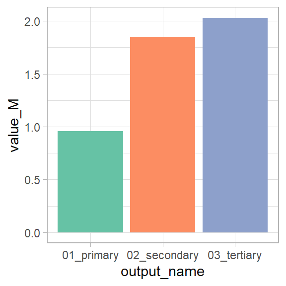
1 industry    01_primary   0.958
2 industry    02_secondary 1.85
3 industry    03_tertiary  2.03
We introduced a method for performing input-output analysis in R.
The calculations shown here have been packaged as econio. The econiodatajp package also lets you fetch an input-output table directly, without having to download and reshape it from e-Stat yourself. As shown below, you can perform the same calculations as above using these packages (note: the jpio package used in an earlier version of this article is no longer maintained and has been replaced by econio/econiodatajp).
# Input-output table: regional
# Dimensions:         output [37], input [37]
# Input:              37 sectors
# Output:             37 sectors
# Import type:        competitive
   output$sector
   <sector>
 1 <industry> 01_Agriculture, forestry and fishery
 2 <industry> 01_Agriculture, forestry and fishery
 3 <industry> 01_Agriculture, forestry and fishery
 4 <industry> 01_Agriculture, forestry and fishery
 5 <industry> 01_Agriculture, forestry and fishery
 6 <industry> 01_Agriculture, forestry and fishery
 7 <industry> 01_Agriculture, forestry and fishery
 8 <industry> 01_Agriculture, forestry and fishery
 9 <industry> 01_Agriculture, forestry and fishery
10 <industry> 01_Agriculture, forestry and fishery
# ℹ 1,359 more rows
# ℹ 2 more variables: input <tibble[,1]>, . <dbl>
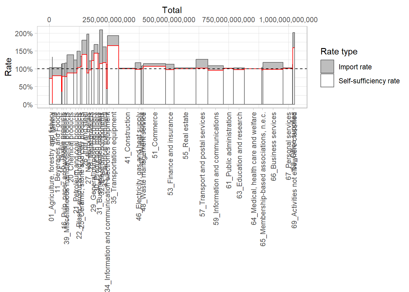
# Skyline chartautoplot(iotable, type ="skyline")
econio doesn’t provide a dedicated function for the economic ripple effect from a specific final demand change. As shown earlier, you can compute it directly by multiplying the Leontief inverse matrix by the final demand change vector.