Calculating the Area of a Circle Using Numerical Integration in R

Note: This article is translated from my Japanese article.

Introduction

I recently learned that the integrate() function in R’s stats package¹ can perform numerical integration of one-dimensional functions. So in this article, referring to this article, I tried calculating the area of a circle using integration.

A function to draw a semicircle

A function that draws a semicircle of radius \(r\) can be expressed as Equation 1. Written in R, this becomes the semicircle() function.

\[ y = \sqrt{r^2 - x^2} \qquad (-r \le x \le r) \tag{1}\]

semicircle <- function(x, radius) {
  sqrt(radius^2 - x^2)
}

Let’s use the semicircle() function we implemented to draw a semicircle with radius \(r = 5\).

radius <- 5
curve(semicircle(x, radius), -radius, radius,
      asp = 1) # Set the aspect ratio to 1:1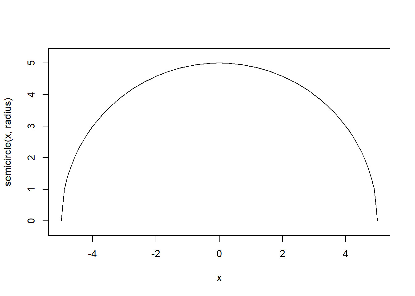

Calculating the area of a circle with numerical integration

Next, let’s use the stats::integrate() function to numerically integrate the semicircle() function we just wrote. For radius \(r = 5\), we can confirm that the integral is approximately equal to the area of a semicircle, \(\frac{1}{2}\pi r^2\).

# Set the radius to 5
radius <- 5
integrate(semicircle, -radius, radius, # Integrate over the range from -radius to radius
          radius = radius)

39.26991 with absolute error < 2.5e-08

pi * 5^2 / 2

[1] 39.26991

Therefore, we can write circle_area_approx(), which approximately computes the area of a circle, as follows (the result of the numerical integration is stored in the value element of the return value of stats::integrate()).

circle_area_approx <- function(radius) {
  out <- integrate(semicircle, -radius, radius,
                   radius = radius)
  out$value * 2
}

circle_area_approx(5)

[1] 78.53982

Finally, let’s compare the approximate values from circle_area_approx() with the theoretical values from circle_area_true() (\(\pi r^2\)) over the range \(1 \le r \le 10\).

The calculation confirms that the approximate and theoretical circle areas are nearly equal.

circle_area_true <- function(radius) {
  pi * radius ^ 2
}

data <- data.frame(radius = 1:10)
data$circle_area_approx <- sapply(data$radius, circle_area_approx)
data$circle_area_true <- sapply(data$radius, circle_area_true)
knitr::kable(data)

radius	circle_area_approx	circle_area_true
1	3.141593	3.141593
2	12.566371	12.566371
3	28.274334	28.274334
4	50.265482	50.265482
5	78.539816	78.539816
6	113.097335	113.097335
7	153.938040	153.938040
8	201.061930	201.061930
9	254.469005	254.469005
10	314.159265	314.159265

Conclusion

We have seen that the stats::integrate() function makes it easy to perform numerical integration of one-dimensional functions.

A note of caution

The stats::integrate() function can also perform numerical integration over the range \(-\infty \le x \le \infty\), but be aware that it may not integrate correctly when given large values such as \(10^{-6} \le x \le 10^6\).

# OK
integrate(dnorm, -Inf, Inf)

1 with absolute error < 9.4e-05

# Not OK
integrate(dnorm, -1e6, 1e6)

0 with absolute error < 0

Footnotes

The stats package is one of the packages that comes with R by default.↩︎